Fusion of multimodal data is far less common than fusion of data from the same sensor type. At present, little work in the literature describes the actual fusion of passive sound and vision. Mak and Allen [29] and Duchnowski et al. [28] describe the integration of lip motion and sound data for improved speech recognition. In related work, Bub, Hunke, and Waibel [51] use visual tracking of a human face to cue an acoustic beamforming algorithm, which reinforces the voice signal from an array of fifteen microphones. Each of these systems assumes that only one person is in the camera view, since they cannot distinguish which person is speaking. Takahashi and Yamasaki [52] demonstrate the calculation of sound source localization by using visual motion data to cue an adaptive FIR filter processing the signal from six microphones. Wasson [49] detects multiple sound targets and visual targets separately, associating them with one another at the symbolic level. Sound targets detected outside the camera field-of-view result in camera motion to confirm the target positions visually. These works suggest that directional sound and directional vision information may be used together for better localization of speech activity.
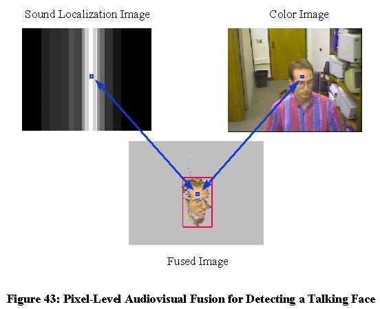
Rather than associating sound and vision at the symbolic level, one may fuse this data at the pixel level. Given a spatially distributed cellular representation of the world such as an image, one may project sound information onto it and detect human activity using sound and image measurements simultaneously. In effect, the detector will look for "noisy" face-colored pixels. Figure 43 illustrates how 1-D sound localization data (normalized onset correlation output) mapped to the same coordinates as the current camera image allows pixel-level fusion of these two sensing modalities. The main objective of this research is to use multimodal data at an early level of processing to improve the reliability of localization of the person speaking. If one combines sound localization evidence supporting the proposition of a location in the world being occupied by a person with visual evidence in support of that location being occupied, a more accurate detector may be designed.
Figure 43: Pixel-Level Audiovisual Fusion for Detecting a Talking Face
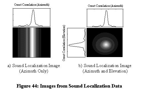
Figure 44: Images from Sound Localization Data
With only two microphones, onset correlation provides a 1-D function of sound power versus azimuth, since interaural delay and azimuth are related by Equation (1). Figure 44a shows this function mapped to a two-dimensional "sound image," where image brightness indicates the level of onset correlation. In this example, it has been assumed that elevation is small enough that each column of pixels relates directly to an interaural delay value. (The actual locus of points defined by a given interaural delay is a hyperbolic cone, but this is approximated as a vertical plane in Equation (1).) If two orthoganal pairs of microphones are used for onset correlation, then sound energy may also be related to elevation. Figure 44b shows how onset correlation plots for azimuth and elevation may be combined to create a 2-D image of sound power. In this illustration, correlation values for elevation and azimuth are multiplied together to form each pixel in the sound image, thus highlighting the area where sound power from each direction intersects. (Onset correlation values from two pairs of microphones are statistically independent between azimuth and elevation. This means that the probability that a sound originates at a given azimuth and elevation may be calculated from the product of the individual azimuth and elevation probabilities for the two onset correlation plots. Multiplication of the raw correlation values between the independent measurements is not exacly the same as multiplying their probability densities conditional on the presense of a sound target, but is close enough for illustration purposes intended in Figure 44.) Only one pair of microphones was available for real-time processing for the implementation done in this research, so only the 1-D sound image is used in the remainder of this dissertation.
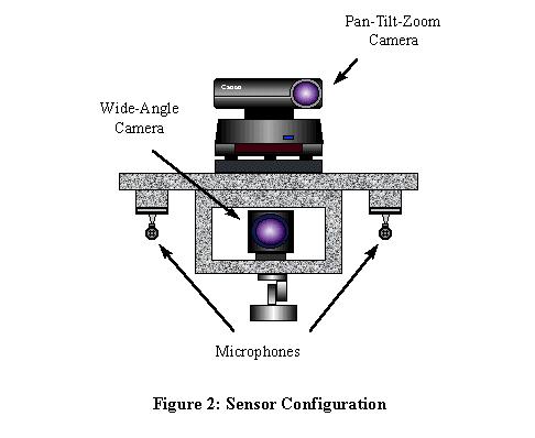
Sound localization and image pixel information both involve the angle at which target data arrives at the sensor. If one positions the cameras and microphones to share the same origin, then these sensors may use the same polar coordinate system. Figure 2 illustrates the placement of the wide-angle camera between the microphones. Naturally, both cameras may not be placed at the origin, so the pan-tilt-zoom camera is mounted about 15 cm above the wide-angle camera. Note also that the camera lens is horizontally offset about 3 cm from the center of the camera, and that the optical axis does not run through the pivot point. At close range, this less-than-ideal geometry adversely affects the accuracy of position measurements and movements, but for more distant targets, it may be ignored. Pixel-level fusion between two cameras, as performed in applications such as stereo vision, requires very precise alignment of optics. Sound localization data, however, is much lower resolution than the image data, requiring less precise alignment for fusion to take place and allowing a common origin to be assumed for each. It will also be assumed that the target's angle of elevation will be small enough that the estimation of sound azimuth will be approximately equal to the visually measured azimuth in polar coordinates.
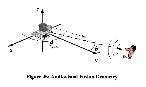
Figure 45: Audiovisual Fusion Geometry
To create a 1-D sound image that is registered with the
current camera image, the pixel column number, m, must be
mathematically related to the corresponding interaural delay,
dm. This requires knowledge of the camera pan angle in radians
(![]() pan), camera field-of-view
in radians (fov), and the image width in pixels (M).
Figure 45 shows the relationship between the camera pan angle, which
is measured with respect to the the x axis, and sound angle,
pan), camera field-of-view
in radians (fov), and the image width in pixels (M).
Figure 45 shows the relationship between the camera pan angle, which
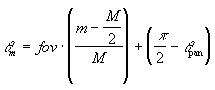
is measured with respect to the the x axis, and sound angle, ![]() m, which is measured relative to
the y axis (relative to the center of the field of view). For a given
image column m, the sound angle
m, which is measured relative to
the y axis (relative to the center of the field of view). For a given
image column m, the sound angle ![]() m is calculated as
m is calculated as
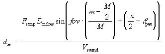
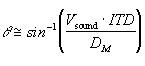
This sound angle is then used to calculate the corresponding interaural delay, dm, as
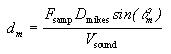
where Fsamp is the sampling frequency (44.1 kHz), Dmikes is the the spacing betwen the microphones (0.30 m), and Vsound is the speed of sound (approximately 344 m/s). A similar calculation could be used for elevation data, if available, using image rows and camera tilt.
Each column of the resulting sound image is set to the value
of the onset correlation, ![]() , for the
corresponding interaural delay. This image provides a measure of
acoustic power relating to each location in the camera image.
However, in order to display the data as a gray-scale image like
Figure 44, it must be normalized by dividing
through by its maximum value. Such normalization is also used to
incorporate the sound data feature into the classifier described in
the next section.
, for the
corresponding interaural delay. This image provides a measure of
acoustic power relating to each location in the camera image.
However, in order to display the data as a gray-scale image like
Figure 44, it must be normalized by dividing
through by its maximum value. Such normalization is also used to
incorporate the sound data feature into the classifier described in
the next section.
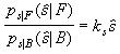
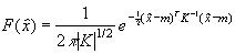
A statistical classifier was designed to classify image pixels as "Talking Face" or "Background" using the color and sound features described in the previous two chapters. From Therrien [66], the decision rule for a two-class minimum Bayes risk classifier is expressed in terms of the probability density likelihood ratio as
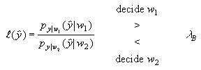 (7)
(7)
where
![]()
The terms ![]() and
and ![]() are the probability densities of
the measurement vector
are the probability densities of
the measurement vector ![]() for classes
w1 and w2, respectively. Pr[w1] and
Pr[w2] denote the prior probabilities of the two classes, and
Cij is the cost of deciding on class wi when
for classes
w1 and w2, respectively. Pr[w1] and
Pr[w2] denote the prior probabilities of the two classes, and
Cij is the cost of deciding on class wi when ![]() is actually from class wj.
is actually from class wj.
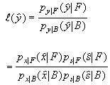
For a "noisy face pixel" detector, the measurement vector
![]() may be broken down into two
vectors:
may be broken down into two
vectors: ![]() , the chromaticity of the pixel
under consideration, and
, the chromaticity of the pixel
under consideration, and ![]() , the onset
correlation strength corresponding to that pixel angle. Sound and
color are assumed to be statistically independent features, allowing
their joint probability density to be expressed as the product of two
independent densities. For the two classes, "Talking Face" (F)
and "Background" (B), one may write these density functions as
, the onset
correlation strength corresponding to that pixel angle. Sound and
color are assumed to be statistically independent features, allowing
their joint probability density to be expressed as the product of two
independent densities. For the two classes, "Talking Face" (F)
and "Background" (B), one may write these density functions as
![]() (8)
(8)
and
![]() (9)
(9)
The probability density function for the chromaticity of face
pixels, ![]() , was defined by a Gaussian
distribution in Equation (6) as discussed in
Chapter 4. The chromaticity density function
for background pixels,
, was defined by a Gaussian
distribution in Equation (6) as discussed in
Chapter 4. The chromaticity density function
for background pixels, ![]() , depends on
the particular room and view where the image was taken. Since this
cannot always be known a priori, it may be approximated by a uniform
distribution in the color space, with a constant density value
, depends on
the particular room and view where the image was taken. Since this
cannot always be known a priori, it may be approximated by a uniform
distribution in the color space, with a constant density value ![]() .
.
The sound onset correlation feature must now be defined. In
the previous section, the onset correlation, ![]() , was related to the image pixel column m by
interaural delay,
, was related to the image pixel column m by
interaural delay,
 (10)
(10)
The cross-correlation value itself is awkward to use directly as a feature for statistical classification since it is highly sensitive to variations in gain and speaker volume. A normalized feature may be found by dividing by the sum of the correlation values over the valid interaural delay range:
 (11)
(11)
Other possible normalizations include scaling by the dynamic range
of ![]() :
:
![]() (12)
(12)
or dividing by the maximum:
![]() (13)
(13)
Since the onset signal value is always non-negative, the cross-correlation value is always non-negative, and thus for all of these functions,
![]() .
.
The probability density functions ![]() and
and ![]() could be
modeled for any of these representations of
could be
modeled for any of these representations of ![]() , and statistics gathered from experimental data to find
the corresponding model parameters. However, a different approach was
used in this work. The likelihood ratio
, and statistics gathered from experimental data to find
the corresponding model parameters. However, a different approach was
used in this work. The likelihood ratio

which represents the degree of belief in the "Talking Face" class
given sound information, should be lowest for ![]() = 0, highest for
= 0, highest for ![]() = 1,
and a monotonically increasing function in between. Since it is
difficult to fully characterize the exact probability density
functions given changes in range to the target and other variables, a
linear approximation for the likelihood ratio may be specified as
= 1,
and a monotonically increasing function in between. Since it is
difficult to fully characterize the exact probability density
functions given changes in range to the target and other variables, a
linear approximation for the likelihood ratio may be specified as
 (14)
(14)
The minimum Bayes risk decision rule in Equation (7) is now rewritten for the talking face detector. Substituting equations (8) and (9) into the expression for the likelihood ratio one obtains:
Next, Equation (6) is substituted for ![]() , kxB is substituted for
, kxB is substituted for ![]() , and
Equation (14) is used to replace the remaining terms, resulting in
the decision rule
, and
Equation (14) is used to replace the remaining terms, resulting in
the decision rule
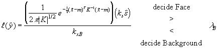 (15)
(15)
Factoring out constants for inclusion in the decision threshold, one obtains
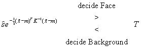 (16)
(16)
where
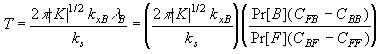
Because the costs Cij, prior probabilities, or constants kxB and ks may not be known, one may determine the decision threshold T empirically by running the system and manually adjusting T until the best detector performance is achieved. This technique was used for this dissertation project, where the number of false positive and false negative classifications were easily observable while the threshold was adjusted.
The addition of the sound localization feature to the face tone information reduces the number of false positive detections of talking face pixels by reducing the likelihood ratio of pixels that do not correspond to the direction of sound. For the binaural case considered in this dissertation, only one direction of sound localization, azimuth, is available, so pixels in the image are biased on a column-by-column basis. This still results in a significant reduction in false positive detections since the image is wider than it is tall and multiple faces usually appear beside one another. Any reduction in the number of pixels marked as skin-colored reduces the number of regions that must be analyzed further to determine their acceptability as face regions. In fact, it reduces the number of segmented regions to the point that the largest blob of detected pixels is almost always the speaker's face.
The Bhattacharyya distance [66] may be used to bound the probability of error on the classifier and quantify the performance benefit of adding the sound feature. The Bhattacharyya distance is a measure of separability between classes based on their probability densities, and is defined as
![]()
A related quantity called the Bhattacharyya coefficient is defined as
![]() (17)
(17)
For a minimum Bayes error classifier (Equation (7) with costs Cij removed) the probability of error is bound by the relation
![]() (18)
(18)
called the Bhattacharyya bound. For the talking face pixel detector, substituting the joint probability densities from Equations (8) and (9) into (17) yields
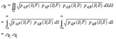
Since ![]() shows the sound
feature's contribution to lowering the bound on the probability of
error.
shows the sound
feature's contribution to lowering the bound on the probability of
error.
A closed form solution for Equation (17) for Gaussian probability densities is given in [66] as
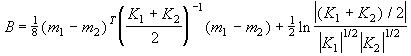
Data from onset correlation experiments was manually sorted into face and background samples, and the feature was generated using Equation (13). The density functions and were matched to Gaussian curves with sample means m1 = 0.7582 and m2 = 0.2785, and sample variances K1 = 0.0439 and K2 = 0.0253, respectively. This resulted in a calculated of 0.4270, meaning that the addition of sound information to the original color classifier reduced the bound on the probability of error by 57.3%. If two pairs of microphones were used in orthogonal directions, one for azimuth and another for elevation, the effect of would be squared, with a total error bound reduction of 81.7%.
For the color feature , the statistics of foreground and background pixel samples in several images were processed to calculate . The chromaticity means for face samples and office background samples were
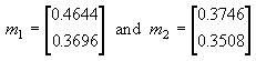
respectively, with covariances
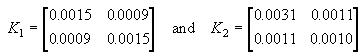
This resulted in a ![]() value of
0.5735. If one assumes that the prior probabilities of face pixels
and background pixels are 1/8 and 7/8, respectively, the
Bhattacharyya bound on the probability of error of is
(1/8)1/2(7/8)1/2(0.5735) = 0.1897 when using color information alone.
When the classifier also incorporates the sound data, the
Bhattacharyya bound drops to (1/8)1/2(7/8)1/2(0.5735)(0.4270) =
0.0810, meaning the classifier will provide the correct answer at
least 91.9% of the time.
value of
0.5735. If one assumes that the prior probabilities of face pixels
and background pixels are 1/8 and 7/8, respectively, the
Bhattacharyya bound on the probability of error of is
(1/8)1/2(7/8)1/2(0.5735) = 0.1897 when using color information alone.
When the classifier also incorporates the sound data, the
Bhattacharyya bound drops to (1/8)1/2(7/8)1/2(0.5735)(0.4270) =
0.0810, meaning the classifier will provide the correct answer at
least 91.9% of the time.
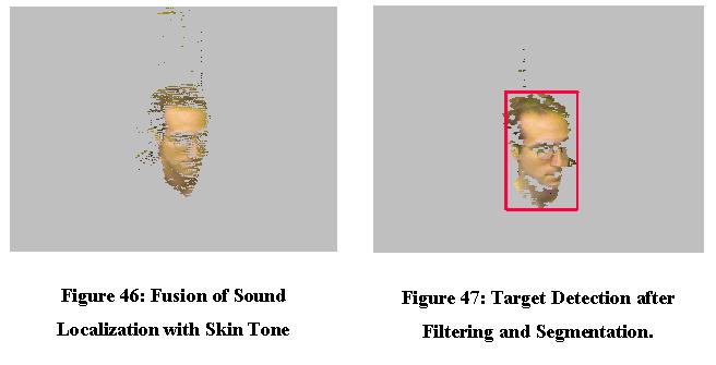
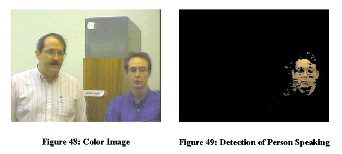
Figure 46 shows the detection of face pixels using both sound and skin tone. Note how many skin-colored background pixels such as those detected in Figure 41 have been eliminated in Figure 46. In this way, sound information is used to simplify the visual task and improve performance. Figure 47 shows a similar frame after 3 x 3 filtering and region-growing to reduce noise and delineate the face region. Figure 48 shows two people within the camera's view, with the person on the right speaking. Figure 49 shows the detected skin-colored face pixels that correspond to the direction of sound. This method allows non-speaking faces to be eliminated from consideration without detecting and processing the regions they occupy.
Figure 46: Fusion of Sound Localization with Skin Tone
Figure 47: Target Detection after Filtering and Segmentation
Figure 49: Detection of Person Speaking
This chapter has demonstrated how audio and visual information may be combined during the classification of pixels. After segmentation and region growing, the next task is to determine which of the remaining regions is a face. One may use size, bounding box aspect ratio, region moments, or other classifiers to make this determination. A person's arm, for example, may appear in the image and take up as much image area as the face. Region moments and bounding box information can be used to dismiss such a region. Ideally, background objects above and below the face will not be skin-colored, simplifying the region selection task. Otherwise, a more sophisticated face detector might be used, such as one based on pattern analysis, or complementary information such as that from an orthogonal microphone pair will be required. For this dissertation project, however, simply choosing the largest segmented region (e.g., the box in Figure 47) was a surprisingly effective means of finding the speaker's face for the requirements of camera control.