1.1: Modeling
ISE 754: Logistics Engineering, Fall 2026
“When in doubt, estimate. In an emergency, guess. But be sure to go back and clean up the mess when the real numbers come along.” — Akin’s Laws of Spacecraft Design1
1. What is logistics engineering?
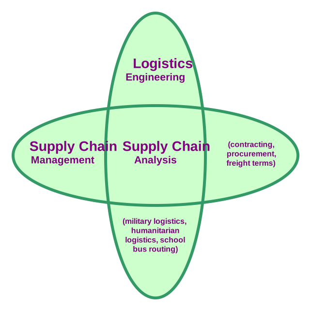
Logistics engineering is the study of the models and methods used to deal with things not being where you want them, when you want them. Topics within logistics engineering include location, transport, networks, and routing, which are used to deal with things not being where you want them, while the topic of inventory is used to deal with things not being available when you want them. As can be seen in Fig. 1, logistics engineering overlaps quite a bit with supply chain analysis. Supply chain management is the study of the processes associated with controlling the materials used in the production of a physical good, and it includes the study of the managerial and legal issues associated with contracting, procurement, and freight transport that are typically studied in a business school, while supply chain analysis refers to the same models and methods used in logistics engineering when dealing with physical goods. Logistics engineering differs from supply chain analysis in that it also deals with systems that are used to produce a service for things like, for example, military operations, humanitarian relief, and school bus routing; it is typically studied in an engineering school.
2. Scope of logistics decisions
The models and methods used to make decisions regarding logistic systems differ with respect to time span over which the decisions will have an impact on the operation of the system. Much more significant and costly effort is put into decisions that will have long-term impact, while the time required to make a decision can be much more important for frequent short-term decisions. The scope of these decisions is traditionally divided into the following three categories:
- Strategic (years): logistics network design; capacity planning.
- Tactical (weeks–year): multi-stage, multi-period, multi-product production and inventory models; transportation planning.
- Operational (minutes–week): scheduling; vehicle routing.
Each scope level is illustrated by a representative problem.
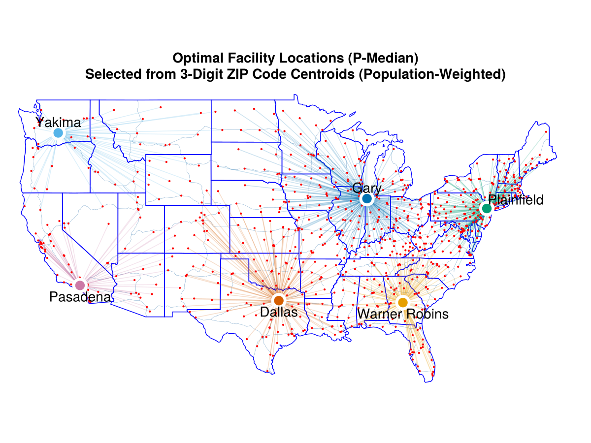
Strategic: logistics network design. A classic strategic logistics problem: place a fixed number of distribution hubs to minimize total weighted distance to customers. Using U.S. 3-digit ZIP code centroids as demand points and population as demand weight, the p-median model selects six hubs that minimize total people-miles.
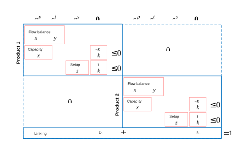
Tactical: production-inventory model. The constraint matrix for a 2-product, multi-period model with setups.
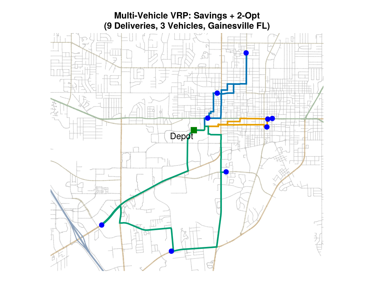
Operational: vehicle routing. A capacitated multi-vehicle vehicle-routing problem (VRP) in Gainesville, FL: three vehicles, each making at most three deliveries, share nine stops from a central depot and return after completing their routes. Stop locations are specified as street addresses and geocoded to coordinates.
3. Modeling: representation and prescription
A logistics study rarely stops at describing a system. The reason to build a model is usually to change the system: to choose a solution that performs better than the system in place. Four terms name the kinds of model involved:
- a model is a representation of the system, detailed enough to predict how it would perform;
- a descriptive model computes a measure of performance with no preference about the outcome, and determines nothing (the guesstimation and mean-value models later in this lecture are of this kind, returning an estimate or an average);
- a feasibility model determines unknowns that must satisfy stated conditions, with no preference among the answers that work;
- an optimization model determines unknowns and adds a preference, an objective, and chooses the answer that performs best. Feasibility and optimization models both prescribe, since each determines something rather than only reporting on it; the distinction that does the daily work is the simpler one, whether a model needs an answer that works or the best one.
Whatever form a model eventually takes, it is written down with keywords, at most the five below, listed in the order they appear in the boxes that follow. A descriptive model uses only the last two. solve for: is what makes a model determine something, and an objective is what makes such a model an optimization, so which of the first two lines appear is what tells the three kinds apart:
- minimize (or maximize): the objective, the preference added to change the system rather than only describe it;
- solve for: the unknowns the model determines, each with what values it may take;
- subject to: the constraints, the conditions any acceptable solution must satisfy; a model with none writes
nonerather than dropping the line, since an unconstrained problem is a finding about it and not an omission; - return: the output of the model, as one thing: a measure of performance for a descriptive model, the decision determined for a model that determines something;
- assumptions: what the model takes as given about the world and its data.
A constraint and an assumption are easy to confuse and do opposite work: a constraint restricts the solution (which answers the model may return), while an assumption restricts the world and its data (what the model takes as given about the setting).
Building the representation is making a model; naming the unknowns and determining them is modeling. The first half is descriptive; the second half is where the decision is actually made.
The vocabulary yields exactly three shapes. Stated with the keywords alone, they are, and the full form is set out in the Model Format Reference for when a model needs more than these five lines2:
Descriptive model
return: …
assumptions:
(a) …
Feasibility model
solve for:
(a) …
subject to:
(a) …
return: …
assumptions:
(a) …
Optimization model
minimize: (or maximize:) …
solve for:
(a) …
subject to:
(a) …
return: …
assumptions:
(a) …
When we later attach symbols to these words and an algorithm to solve them, the work of the lectures that follow, a prescriptive model with a numeric objective and algebraic constraints becomes a mathematical program. That is one form a model can take, the most common in logistics, but not the only one; a model may instead be solved by a custom procedure, by simulation, or by direct calculation. The vocabulary above is what stays fixed across all of these forms.
A firm’s goal is to maximize profit, the difference between revenue and cost, but its production and logistics activities are typically handed a specified demand to meet. When the quantity q to be served is fixed and its price P does not depend on how the system is configured, the revenue P\,q is a constant, so maximizing the profit P\,q - C, the revenue less the cost C, is the same as minimizing the cost C. Production therefore contributes to the overall goal of maximizing profit by meeting the specified demand at the lowest possible cost, which is why most logistics problems are posed as cost minimizations.
Because the words come before any symbols, the description of a model is something to read and check on its own: whether its objective, its constraints, and the solution it returns match the decision actually faced, before trusting whatever machinery later produces a solution. We return to this habit of checking once those tools enter in the lectures that follow.
The three problems from the previous section are each a model in this sense. Stated with the common vocabulary, what they share beneath their different time scopes becomes visible.
A model with an objective prescribes; a model without one only describes. The keyword is the whole difference.
The strategic problem chooses where to put a fixed number of hubs; Fig. 2 shows the solution it selects.
minimize: total population-weighted distance (people-miles) from the demand points to the hubs that serve them
solve for:
(a) which six of the candidate locations to open;
(b) which hub serves each demand point.
subject to:
(a) assignment: every demand point is served by exactly one of the six hubs.
return: hub plan: the six locations opened and the hub serving each demand point
assumptions:
(a) demand is located at the 3-digit ZIP code centroids, weighted by population;
(b) number of hubs is fixed in advance, here six.
More hubs, or better-placed ones, would cut the distance; here the count is fixed at six, so only the placement and the assignment are open.
The tactical problem plans production and inventory over time; Fig. 3 writes it out as a constraint matrix, its rows the constraints and its columns the decisions. (What the figure labels setup is a startup cost: it is paid once when a product’s production begins, not in every period it continues.)
minimize: total cost over the planning horizon: production, inventory-holding, and startup costs
solve for:
(a) how much of each product to make in each period, a non-negative quantity;
(b) how much of each product to hold at the end of each period, a non-negative quantity;
(c) whether each product is in production in each period, yes or no.
subject to:
(a) demand: each product’s demand is met every period;
(b) capacity: production stays within capacity every period;
(c) startup: a product incurs a startup cost when its production begins, not in every period it continues.
return: production-inventory plan: what to make and what to hold, by product and period
assumptions:
(a) demand for each product in each period is known;
(b) each product’s price is fixed, independent of the plan.
Keeping a product in production avoids paying to start it up again, but holding the resulting inventory has its own cost; and the two products compete for the same capacity, so periods and products cannot be planned in isolation.
The operational problem routes vehicles for a single day of deliveries; Fig. 4 shows the routes it produces.
minimize: first the number of vehicles used, then, among the solutions that use the fewest, the total distance traveled
solve for:
(a) how many vehicles to use;
(b) which deliveries each vehicle makes, and in what order.
subject to:
(a) coverage: every delivery is made exactly once;
(b) capacity: each vehicle makes at most three drop-offs.
return: day’s routing plan: the vehicles used and the ordered stops of each
assumptions:
(a) all routes start and end at the single central depot;
(b) travel distance between every pair of stops is known.
An extra vehicle, with its driver, fuel, and capital, costs far more than the miles a tighter route would save, so the fleet is shrunk first and distance only breaks ties. This reverses the usual statement of the problem, in which distance is taken as the sole objective.
These three models are stated only at the level of the decision each one makes. Later lectures attach the symbols, the data, and the Julia that turn a model into something runnable. How much detail a model needs, and how much effort solving it takes, is the subject of the next section.
4. Levels of modeling
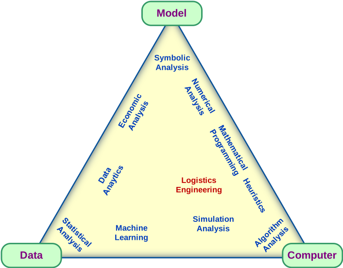
A model is a representation of a real system whose parts and relationships are just detailed enough that it can be used to predict how the system would perform under conditions that have not been tried, and to determine what to do without experimenting on the system itself. Fig. 5 shows a variety of different methods of analysis in relationship to the degree to which they focus on the three elements of the model itself, the data used in making decisions, and the computational effort needed to make decisions. While logistics engineering utilizes all of these different methods of analysis, they tend to focus more towards the computational issues due to the complex interactions of the different elements in most logistics systems.
The preferred modeling approach is to use the simplest (least costly) model necessary to select between multiple alternatives, taking into account the time of the analyst to construct the model and to make decisions using the model. In order of increasing cost and complexity, the following are different levels of modeling used in logistics engineering:
Modeling levelsincreasing cost & complexity ↓
- Guesstimation (order of magnitude)
- Mean value analysis (linear, ±20%)
- Nonlinear models (incl. variance, ±5%)
- Simulation models (complex interactions)
levels 0–3 · course toolkit
- Prototypes / pilot studies
- Build / copy / do and then tweak it (evolutionary approach)
The first four levels are the course’s modeling toolkit, each developed where it is first needed: guesstimation (level 0) in Sec. 5 and mean value analysis (level 1) in Sec. 6 below, then the nonlinear models (level 2) and simulation (level 3) in Lecture 1.3 (Sec. 6 and Sec. 7 there), where estimating the performance of a production system first demands them. Levels 4 and 5 step beyond modeling altogether: rather than represent the system, they build some version of it, a prototype or pilot study testing the design at small scale, and build-then-tweak evolving the real system in place. They are the most costly and the most faithful, the recourse when a system resists representation. The recourse is real: when Intel brings a new high-volume semiconductor fab online, the new factory is built as an exact copy of a working one, “down to the finest detail,” under the company’s Copy EXACTLY! methodology, used for the start-up of its fab in Leixlip, Ireland.3 The reason is the same logic taken to its limit: a fab’s process steps interact so intricately, down to barometric pressure and the length of an electrode cooling hose, that “the only way to guarantee you will always get the same results … is to copy the configuration exactly.” Building something outright, with no modeling first, can be the easy path, but also a costly one. Delco, a General Motors automotive-parts operation, treated every capacity decision as disposable, buying machines and replacing them a few months later when they disappointed; it mistook flexibility for strategy, and within a few years it had failed.4 Levels 4 and 5 receive no further development in this course.
5. Level 0: Guesstimation
Guesstimation can be used to estimate data or system performance for which there is no easy way to model. Rather than saying “I don’t have a clue,” It can be used to get an estimate at least within an order of magnitude of the correct answer. It is the failsafe modeling technique. An order-of-magnitude estimate is also the first check on any elaborate result. A complicated model, or an answer returned by an AI assistant, is judged plausible or suspect by comparing it against a quick, independent guess; a ballpark figure solved by hand is what reveals whether a machine-produced number is even in the right range. It is often hard to estimate a parameter X directly but easy to estimate reasonable lower and upper bounds (LB and UB). Since LB and UB are usually orders of magnitude apart, the arithmetic mean over-weights UB; the geometric mean is a logarithmic average and gives a more reasonable estimate:
\text{Geometric Mean} = \sqrt{\text{LB}\cdot\text{UB}}
For example, how many people can be crammed into a car? more than 1, less than 100: the average 50 is too high, but the geometric mean 10 is reasonable. What if LB is 0? Then the geometric mean is 0 as well, so a zero lower bound is replaced by the smallest value the quantity could realistically take.
Fermi problems (named after the physicist Enrico Fermi) are inspired guesses about quantities that seem almost impossible to determine given limited data. Solving one involves “reasonable” (±10%) guesstimation of the input parameters and back-of-the-envelope approximations. The goal is an answer within an order of magnitude of the correct answer (a zeroth-order approximation). It works because of decomposition: the over- and under-estimates of each parameter tend to cancel out as long as there is no consistent bias. The reason ten coin flips land nearer the average than a single flip does is the same phenomenon at work here, a small instance of the law of large numbers. The value of such an estimate is speed: a roughly-right answer available at once, weeks before the data for an exact answer could be assembled, and often the only way to estimate data that is not publicly available.
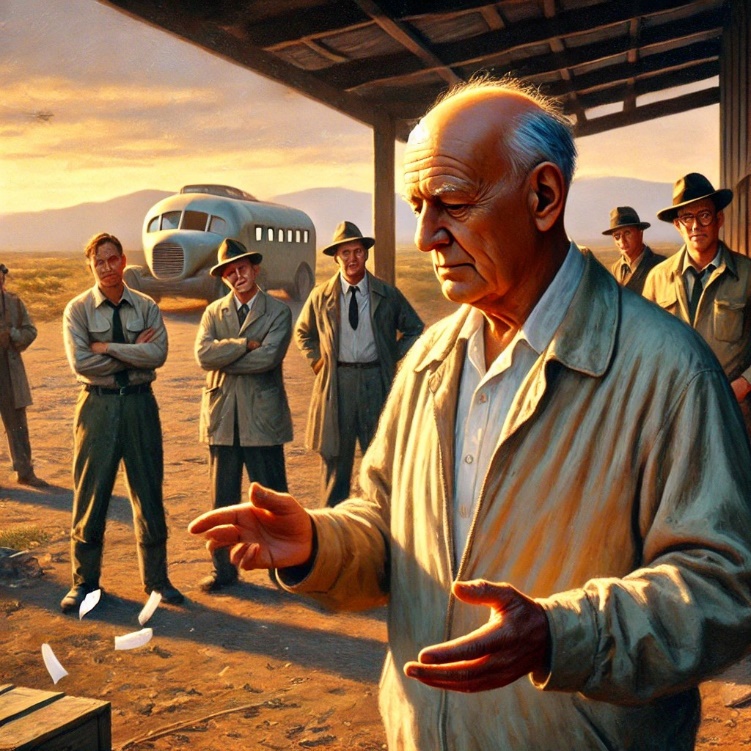
At the Trinity test (see Fig. 6), Enrico Fermi estimated the blast’s yield by dropping scraps of paper as the shock wave passed and measuring how far they were carried. His figure, about 10 kilotons, landed within an order of magnitude of about 21 kilotons, the yield later established by measurement, the accuracy a guesstimate aims for.
Example 1: McDonald’s restaurants
Estimate the number of McDonald’s restaurants in the U.S. (assume no internet).
“Reasonable” guesstimates can be made for all of the parameters except customer demand, so the geometric mean of the estimated lower and upper bounds on demand is used. The actual number of McDonald’s restaurants in the U.S. as of 2013 was 14,267,6 around 11% below the estimate. A key assumption is that the number of restaurants has reached market saturation, so the entire U.S. population can be used as the customer base. A single-leap guess at the store count would span from perhaps 50, one per state, to hundreds of millions, one per person, a bracket whose guesstimate is wrong by orders of magnitude; decomposing the estimate into individually reasonable factors is what can make the result more accurate.
All parameters except per-capita demand can be guesstimated directly. For demand, take a lower bound \text{LB} = 1 order/person-yr and an upper bound \text{UB} = 350 order/person-yr (one order per person-day over a 350-day operating year), and use their geometric mean:
f = \sqrt{\text{LB}\cdot\text{UB}} = \sqrt{1 \times 350} \approx 18.7\ \text{order/person-yr}
With U.S. population q = 300,000,000 persons, operating hours H = 16 hr/day, per-store rate r = 1 order/store-min, and the geometric-mean demand f ≈ 18.7 order/person-yr from above, the store count follows from one idea: work out how many orders the country places each day, work out how many one store can fill in a day, and divide. Follow the units on the right of each line: orders per year become orders per day, and finally cancel to leave a store count.
Annual U.S. demand. Every person places about f orders a year, so all q of them together place population times the per-person rate:
q\,f = (3\times10^{8})(18.7) \approx 5.6\times10^{9}\ \text{order/yr}
Daily U.S. demand. Spreading that evenly across the 365 calendar days of the year (the 350-day figure above was only a per-person ordering rate, not a store’s open days) turns the yearly figure into a daily one:
\frac{q\,f}{365} = \frac{5.6\times10^{9}}{365} \approx 1.5\times10^{7}\ \text{order/day}
What one store can serve. Now switch from the whole country to a single store. Open H hours a day and filling r order every minute, its daily capacity is (the 60 converts hours to minutes):
H \times 60 \times r = 16 \times 60 \times 1 = 960\ \text{order/store-day}
Number of stores. It takes enough stores to cover the national daily demand, so divide the country’s orders per day by one store’s capacity; the order-per-day units cancel and leave a pure store count:
\frac{q\,f/365}{H \times 60 \times r} \approx 16{,}017\ \text{stores}
Estimated number of U.S. stores ≈ 16,017
Example 2: Truckloads per week
A big-box home improvement store (like a Lowe’s or Home Depot) receives shipments from its distribution center (DC), where each shipment consists of the entire contents of a tractor trailer. Estimate how many truckloads of product a typical store receives from its DC during an average week.
As in Ex. 1, the weekly truckload count is not guessed in one step. It is broken into the pieces that each must occur on the way to a received truckload, so that an over-estimate of one piece tends to be offset by an under-estimate of another when the pieces are multiplied together. Three of the pieces are uncertain enough to bracket and estimate by their geometric mean; the other two are known closely enough to fix directly.
Reasonable values for the cube of a full truckload and the store’s daily operating hours are assumed based on prior knowledge. Three pieces are uncertain, so each is bracketed by a low (LB) and a high (UB) and estimated by the geometric mean of the two. Two are easy to bracket: the number of receiving lanes running at once (1 to 10) and the orders each lane handles per hour (10 to 60). The order cube needs its bounds worked out first: a small parcel is a 2-inch cube, (2 \times 2 \times 2)/12^3 = 0.0046 ft³, and a bulky load is 4 \times 5 \times 10 = 200 ft³. Those low and high values go into Table 1 alongside the others.
| Parameter | LB | UB | Estimate | Units |
|---|---|---|---|---|
| Cube per truckload | 3,000 | ft^3/TL | ||
| Cube per order | 0.0046 | 200 | 0.96 | ft^3/order |
| Number of lanes operating | 1 | 10 | 3.16 | lanes |
| Orders per lane-hr | 10 | 60 | 24.5 | orders/lane-hr |
| Operating hours per day | 15 | hr/day |
Composing the parameters, one operation at a time, carries the estimate down to a weekly truckload count. Each calculation in Table 2 is written in the units of the quantities it multiplies or divides, so the units themselves do the bookkeeping: the shared units cancel and the result comes out in the units that remain.
| Quantity | Calculation | Estimate | Units |
|---|---|---|---|
| Orders per day | (lanes) × (orders/lane-hr) × (hr/day) | 1,162 | orders/day |
| Cube per day | (ft^3/order) × (orders/day) | 1,118 | ft^3/day |
| TL per day | (ft^3/day) / (ft^3/TL) | 0.373 | TL/day |
| Days between TL | 1 / (TL/day) | 2.68 | day/TL |
| TL per week | (TL/day) × 7 | 2.61 | TL/wk |
Should the result be rounded to a whole number of truckloads? No, keep the fractional 2.61 TL/week; why the fractional part is kept is taken up in a later lecture.
Estimated truckloads received ≈ 2.61 TL/week
6. Level 1: Mean value analysis
Mean value analysis: a modeling approach that replaces variability with averages; it is useful when the law of large numbers and pooling cancel fluctuations out, but is limited when variability or nonlinear effects matter.
When is it OK to use mean value analysis?
- May be OK for many strategic and some tactical modeling applications.
- Rarely OK for operational modeling, where the outcome is driven by short-run variability rather than by the average.
Example 3: Commuting
The following are (sorted) travel times of a dentist from her home in Raleigh to her office in Chapel Hill each morning for a typical week: 40, 40, 45, 75, 90 minutes.
Example 3(a): Average, median, mode, and monthly commuting hours
What is the average? Median? Mode? Assuming similar times for the trip home, how many hours per month does she spend commuting?
For the five times 40, 40, 45, 75, 90: the average is 58 min, the median is 45 min, and the mode is 40 min. Assuming 20 commuting days per month and a round trip, the monthly commuting time follows from the scalability of the mean (below).
Average 58 min, median 45 min, mode 40 min; \approx 38.67 hr/month commuting.
Scalability of the mean: the mean scales the total up or down for a different count n,
\bar{x} = \frac{\sum_{i=1}^{n} x_i}{n} \;\Rightarrow\; n\,\bar{x} = \sum_{i=1}^{n} x_i \;\Rightarrow\; n'\,\bar{x} \approx \sum_{i=1}^{n'} x_i .
For the commuting question, the round-trip monthly total, twice the one-way mean \bar{x} over the month’s n' commuting days, works out to:
\frac{2\,n'\,\bar{x}}{60} = \frac{2(20)(58)}{60} \approx 38.67\ \text{hr/month}
Scaling is only valid when
- the data is stationary (no trend, seasonality, or structural changes), and
- the mean is used in a linear function (because of Jensen’s inequality).
The mean is also not valid under trend, seasonality, or a one-time structural change. Making a series stationary before averaging, and why stationarity is the key assumption behind the factory-physics formulas, is taken up in detail in Lecture 1.3, System Performance Estimation.
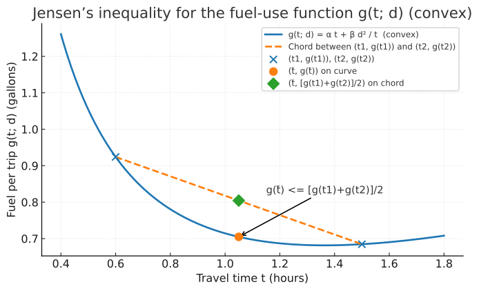
For nonlinear functions g, applying g to the mean of the values is generally not equal to taking the mean of g applied to each value:
g(\bar{t}) \ne \frac{1}{n}\sum_{i=1}^{n} g(t_i) .
Fuel use from travel time (fixed distance). Let d be the trip distance (miles), the average speed v = d/t mph, and the fuel-consumption rate r(v) (gallons/hour)
r(v) = \alpha + \beta v^2,
where \alpha = 0.275 gal/hr (idle/AC fuel use), \beta v^2 is the aerodynamic-drag term, and \beta = 5.16e-04 gal/(hr·mph²).7 The fuel (in gallons) for one trip of duration t is
g(t; d) = t\,r\!\left(\frac{d}{t}\right) = \alpha t + \beta \frac{d^2}{t},
which is nonlinear (convex) in t because t appears in the denominator.
Example 3(b): Weekly fuel usage (Jensen’s inequality)
Determine the weekly fuel usage, illustrating that fuel use is a nonlinear function of travel time, so the mean travel time cannot simply be plugged in.
Five commutes per week, d = 30 miles, travel times (minutes) each way: 40, 40, 45, 75, 90.
| Trip | Time (min) | Time (hr) | Gallons g(t;30) |
|---|---|---|---|
| 1 | 40 | 0.667 | 0.880 |
| 2 | 40 | 0.667 | 0.880 |
| 3 | 45 | 0.750 | 0.825 |
| 4 | 75 | 1.250 | 0.715 |
| 5 | 90 | 1.500 | 0.722 |
| Sum | — | — | 4.023 |
Summing the five trips (Table 3) gives 4.023 gal, but using the average travel time (the average-time method, 5\,g(\bar t) with \bar t = 58 min) gives only 3.731 gal, an underestimate of \approx 0.291 gal (about 7.2%), which is exactly the Jensen gap for a convex g.
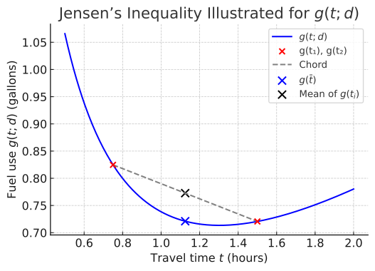
Total weekly fuel \approx 4.023 gal; the average-time method gives 3.731 gal, underestimating by \approx 0.291 gal (7.2%).
Ex. 3 contrasts two uses of the mean. When the quantity of interest aggregates linearly (the total monthly commuting time is just the number of trips times the average trip), the mean is exactly scalable and the estimate is reliable. When the quantity depends nonlinearly on the same data (weekly fuel is a convex function of travel time), plugging the average travel time into the function underestimates the true total by the Jensen gap. The working rule is that a mean may stand in for the data when the quantity of interest is a linear function of stationary values, but not when that function is nonlinear, where the spread of the data itself changes the answer.
The same convexity carries a second lesson. Because g curves upward it has a lowest point: in Table 3 the 75-minute trip burns the least fuel of the five and the 90-minute trip a little more, since driving faster than the most fuel efficient speed spends more fuel fighting drag while driving at slower speeds spends more idling. A convex objective always has a single optimal interior value; a linear objective has no such value, more is always better or worse. Solutions for linear objectives can only be found by bounding the possible values with constraints.
Example 3(c): When should she leave?
When should the dentist leave home each morning to arrive on time?
There is no single answer, and the reason ties straight back to the modeling vocabulary of Sec. 3: the question has no answer until an objective is chosen. A list of travel times is only descriptive; a departure time is a decision, and a decision needs a preference to select it, which is exactly what makes a model prescriptive.
Different objectives give different departure times, each encoding a different tolerance for being late:
- Leave at the mean (about 58 min before the appointment): on time on an average day, but late on any slower-than-average day, which here is nearly half of them.
- Leave for the worst case (90 min before): almost never late, but time is wasted on every ordinary day.
- Leave to be on time a target fraction of days (say 95%): budget enough time to cover all but the slowest one-in-twenty mornings.
Which objective is right boils down to a single question: how costly is it to be late? Being willing to run late one day a week is a very different standard from one day in twenty, and the two imply very different departure times. Determining it means weighing the cost of arriving late against the cost of arriving early and waiting, and the answer stays undecided until those costs are named.
Notice what the mean cannot do here. Mean value analysis knows only the average travel time; it says nothing about how often the trip runs long, which is exactly what a late-arrival objective turns on. The question needs the whole distribution of travel times and its tail, a richer stochastic model than a single average provides. That is the province of the nonlinear (level 2) and simulation (level 3) models of Lecture 1.3: mean value analysis is simply not the right tool for this problem.
Example 4: Pizza delivery distance
A pizza shop delivers to customers located within 3 miles of the shop. Estimate the average round-trip distance of a delivery, then, because the geometry here is simple enough, compute it exactly and compare.
The quantity wanted is a single performance measure, with nothing to choose, so this is a descriptive model: it has a return and its assumptions, but no objective.
return: average round-trip distance of a delivery
assumptions:
(a) every customer lies within the 3-mile delivery radius;
(b) round trip is exactly twice the one-way distance.
Example 4(a): Guesstimate
Rather than guess the round-trip distance in one step, break it into the smallest piece that has to be guessed and use an exact relation for the rest. The one-way distance lies between a lower bound of 1 mile (it cannot be 0) and the 3-mile radius, so its geometric-mean guesstimate is
d_\text{one-way} = \sqrt{\text{LB}\cdot\text{UB}} = \sqrt{1\cdot 3} = \sqrt{3} \approx 1.73\ \text{mi}.
A round trip is exactly twice as far, with no further uncertainty:
d_\text{round} = 2\,d_\text{one-way} = 2\sqrt{3} \approx 3.46\ \text{mi}.
Guessing the round trip directly would instead bracket it between 1 and 2\times 3 = 6 miles, giving the poorer estimate \sqrt{1\cdot 6} = \sqrt{6} \approx 2.45 mi. Decomposing is better for two reasons. In general, breaking a guesstimate into the smallest independently estimable pieces lets the over- and under-estimates of each piece cancel rather than compound. Here it also narrows the range: by guessing only the one-way distance and using the exact fact that a round trip is twice as long, no uncertainty is introduced where the relationship is already known.
Average round-trip distance ≈ 3.46 mi
Example 4(b): Exact average distance
Compute the exact average round-trip distance, and compare it with the guesstimate.
The guesstimate barely used the shape of the service area. An exact answer needs much more, and rests on two assumptions the guesstimate did not: the service area is exactly a disk of radius R = 3 mi centered on the shop, and customers are uniformly distributed over it, every location equally likely (Fig. 9). Both are idealizations, since real delivery zones are irregular and demand clusters, but together they make the average distance exactly computable.
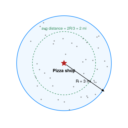
Under those assumptions the average one-way distance works out to \tfrac{2}{3}R = 2 mi, so the average round trip is \tfrac{4}{3}R = 4 mi. The one-line integral behind these numbers is given below.
Under uniform demand the chance a customer lies within distance r of the shop is the fraction of the disk’s area inside radius r:
\Pr(d \le r) = \frac{\pi r^2}{\pi R^2} = \left(\frac{r}{R}\right)^2, \qquad 0 \le r \le R,
so the one-way distance has density f(r) = 2r/R^2 (the derivative of the area fraction), and its mean is
\bar d_\text{one-way} = \int_0^R r\,f(r)\,dr = \frac{2}{R^2}\int_0^R r^2\,dr = \frac{2}{R^2}\cdot\frac{R^3}{3} = \frac{2}{3}R = \frac{2}{3}(3) = 2\ \text{mi}.
A round trip is twice as far, \bar d_\text{round} = \tfrac{4}{3}R = 4 mi.
The guesstimate of part (a), 3.46 mi, lands within about 13% of the exact 4 mi, close enough to act on and a reassuring check on the method. The lesson is not that guesstimates are always this accurate, but the reverse: here we can check because the geometry is simple, while in most real problems no closed-form exists and a guesstimate (or a simulation) is the only answer available. The exact result is the luxury; the bracket is the tool that always works.
Exact average round-trip distance = \tfrac{4}{3}R = 4 mi (vs. 3.46 mi from the guesstimate)
7. Getting started: Claude Code and the toolchain
Course toolchain
Three open-source tools make up the course environment, each introduced in Lecture 1.2:
- Julia, the computational language: fast like C++/Fortran, simple like Matlab/Python (Sec. 1).
- VS Code, the editor, where a
.jlscript runs a line at a time against a live Julia session (Sec. 1.1). - Claude Code, the AI agent, run from the terminal inside VS Code (Sec. 2).
The LLM removes the syntax barrier, so effort goes to modeling rather than to writing code. Because the AI can be confidently wrong, its output must be verified, and verification is the skill the course certifies (Sec. 3).
Bootstrap (demoed in class, written to follow at home)
Install Claude Code first, by hand; it then installs everything else. State a goal, approve what Claude Code proposes, confirm the result: that loop runs all semester. Each step ends with what success looks like. Anything already on the machine is fine, tell Claude Code and it verifies instead of reinstalling. Commands and links are current as of August 2026 and refreshed each semester.
1. Get the claude command. Claude Code needs a Pro, Max, Team, Enterprise, or Console account; the free plan does not include it.8 Open a terminal, on Windows by pressing the Windows key and typing PowerShell, on macOS with Cmd+Space and Terminal, and run the installer for that platform:9
Success: claude --version prints a number followed by (Claude Code). If it says the command is not found, open a new terminal first, since the installer changes the PATH.
The Claude desktop app is a separate download and is not what is needed here. The two share one login, so having the app means being signed in already, but the command above is still required.10 On Windows, Git for Windows is recommended rather than required: with it Claude Code can use a Bash shell, and without it Claude Code uses PowerShell instead.11
2. Let Claude Code install the rest. Everything else, Git, VS Code, its extensions, Julia at the pinned version, and the course packages, is installed by Claude Code following a written procedure the course supplies. Follow SETUP.md, which is four short human steps; it detects what is already on the machine and installs only what is missing, so nothing is removed or reconfigured. It lives in the course materials repository, which the setup clones; nothing needs downloading by hand.
Success: the last step runs a check of eleven things and prints READY, saving the output to ISE754/bootstrap-report.txt.
READY is the smoke test of the whole chain: the tools are installed, the pinned Julia runs, and the course’s packages load. It is also the first instance of something this course returns to constantly, which is confirming a result mechanically rather than trusting that it looks right.
If a step fails, paste the error into Claude Code and let it fix it. Recovering with the agent is the course’s method, met a week early, and the check names which of the eleven failed so there is something specific to paste.
“Claude Code requires a Pro, Max, Team, Enterprise, or Console account. The free Claude.ai plan does not include Claude Code access.”12 The course assumes at least the Pro plan (the individual subscription); Max is Pro with higher limits, Team and Enterprise are organizational, and a Console account bills API use pay-as-you-go. Prices: https://claude.com/pricing.
claude “not recognized”?
Nothing needs removing: SETUP.md probes for each tool and verifies what is present instead of reinstalling it (the Julia VS Code extension finds an existing Julia automatically13). If claude is “not recognized”, the installer’s PATH change has not reached the open terminal yet: close it and open a new one.
8. How the course’s files move
Section 7 installed git, or confirmed it was already present, without saying what it is for. Git is a version-control system: it records a folder’s history rather than only its present contents. Each saved change is a commit, carrying a message, an author and a timestamp, so the question “what changed, and when” has an answer that reading the current file cannot give. That property is used directly in Lecture 1.2, and it is the reason the course keeps its material this way rather than as files passed around.
The practical use here is narrower: git is how material arrives and how work goes back. Three folders sit side by side inside the course folder, and Fig. 10 places them against everything else the course touches.

materials/holds each lecture’s companion script, the data those scripts read, and the pinned Julia environment. It is received, not edited.handouts/holds the homework, projects and study guides. It is also received, and it stays empty until the first homework is assigned.work/is the one written in, and it is what gets submitted.
Three operations cover all of it. git pull brings down whatever has been added to materials/ or handouts/. git push sends the contents of work/ to a private repository readable only by its author and the teaching staff. And feedback on submitted work is written back into that same repository as commits, so it arrives by git pull too, and it announces itself only once that repository’s notifications are switched on.
None of this is needed yet. The first submission is due at 8:00 pm on Monday 24 August, and the full procedure, including the notification setting, is in SUBMITTING.md in the course materials repository.
Assignment (due before class 2)
Complete the setup through step 5, ending with the check reporting READY. Two things then go into Moodle: the entire contents of bootstrap-report.txt, and separately, a short answer in plain prose to what failed, what was done about it, and how the fix was confirmed, for which “nothing failed” is a complete answer. That second answer is typed into Moodle rather than produced by the setup, because everything in the report was generated and that answer is not. A NOT READY report is also worth submitting: knowing what broke, across the class, is what the second meeting is built on. Claude Code needs a paid Anthropic account (Pro or better, see the account note above), so arrange that before starting.
Endnotes
Akin’s Laws of Spacecraft Design (Aug 17, 2023), blog.matt-rickard.com.↩︎
Model Format Reference. It covers the cases these five lines do not reach: when a slot is legitimately empty, how a model written in words descends to symbols and then to code, and how competing approaches to one problem are told apart.↩︎
C.J. McDonald, “The Evolution of Intel’s Copy EXACTLY! Technology Transfer Method,” Intel Technology Journal, Q4 1998, https://www.intel.com/content/dam/www/public/us/en/documents/research/1998-vol02-iss-4-intel-technology-journal.pdf (the full Q4 1998 issue; accessed July 2026). The stated philosophy: “everything which might affect the process, or how it is run is to be copied down to the finest detail, unless it is either physically impossible to do so, or there is an overwhelming competitive benefit to introducing a change.” McDonald served as manufacturing manager for the start-up and ramp of Intel’s high-volume fab in Ireland.↩︎
Based on a personal conversation with a former student employed at Delco, in Ohio, 1998.↩︎
Image generated with DALL·E.↩︎
Source: “Number of McDonald’s restaurants in North America in 2012 and 2013, by country,” Statista.↩︎
Fuel-use data: \alpha is the average of compact (0.16 gal/hr) and large (0.39 gal/hr) sedan idle consumption, Fact #861 (2015); Bifulco, Galante, Pariota & Spena, “A Linear Model for the Estimation of Fuel Consumption…,” Sustainability 7(10), 2015.↩︎
“Quickstart,” Claude Code documentation, https://code.claude.com/docs/en/quickstart (accessed August 2026).↩︎
“Quickstart,” Claude Code documentation, https://code.claude.com/docs/en/quickstart (accessed August 2026). The native installer commands, the
claude --versioncheck, the note that a new terminal may be needed, and the Git-for-Windows recommendation are all from its Step 1.↩︎“Quickstart,” Claude Code documentation, https://code.claude.com/docs/en/quickstart (accessed August 2026). The native installer commands, the
claude --versioncheck, the note that a new terminal may be needed, and the Git-for-Windows recommendation are all from its Step 1.↩︎“Quickstart,” Claude Code documentation, https://code.claude.com/docs/en/quickstart (accessed August 2026). The native installer commands, the
claude --versioncheck, the note that a new terminal may be needed, and the Git-for-Windows recommendation are all from its Step 1.↩︎“Advanced setup,” Claude Code documentation, https://code.claude.com/docs/en/setup (accessed July 2026).↩︎
“Getting Started,” Julia in VS Code documentation, https://www.julia-vscode.org/docs/stable/gettingstarted/ (accessed July 2026).↩︎