allocate (generic function with 1 method)2.3: Multifacility Location–Allocation
ISE 754: Logistics Engineering, Fall 2026
Where to locate, whom to serve: two easy questions, one hard problem.
In a multifacility location problem, the number of NFs to be located can either be specified or can be determined as part of the location procedure. When the number of NFs is specified, the allocation of EFs to NFs can either be given or determined as part of what is then termed a location–allocation problem. If the NF-to-EF allocations are given and there are no interactions between the NFs, then the multifacility problem reduces to a series of single-facility location problems. The location–allocation problem remains difficult even when there are no interactions between the NFs because of the need to determine the allocations.
Locating distribution centers is the most common multifacility location problem, and in the terms just set out it is a location–allocation problem: the number of DCs is either specified or determined as part of the procedure, their allocation of customers is determined rather than given, and there are typically no interactions between the DCs themselves. Most facilities are sited against a long list of considerations, of which transport is only one, but a DC exists to move goods, so its location is close to a pure transport decision. Each customer is normally served by a single DC, and which one that is depends on where the DCs are, so the location and the allocation have to be determined together.
1. Allocation
Allocation problem
Before any facility is moved, there is a smaller problem worth isolating: given where the NFs already are, which one serves each EF, and what does that cost? This is the allocation problem, and it is the inner step of everything that follows.
What makes it an allocation problem is that an EF need not be served by every NF. Where the NFs hold duplicate product, as distribution centers do, the sensible arrangement is for each to serve the EFs nearest it. That is a property of the application rather than of the model: were the NFs suppliers of different inputs instead, each EF would draw from all of them and no allocation would be left to determine.
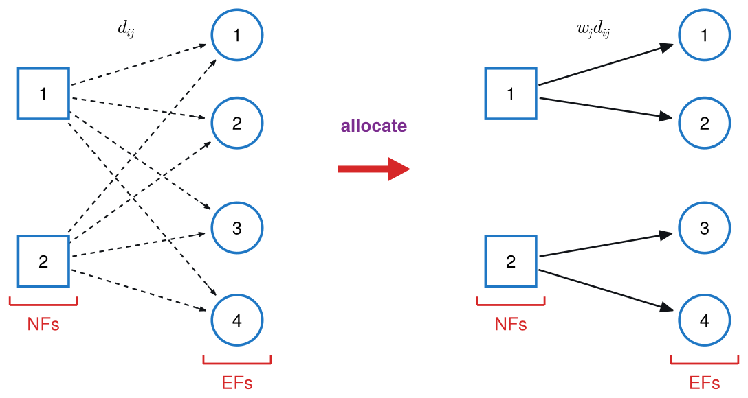
Fig. 1 is the step itself: on the left every NF could reach every EF, and on the right each EF keeps only the link to the NF nearest it.
minimize: total weighted distance from each EF to the NF that serves it
solve for:
(a) NF serving each EF, one of the n NFs for each of the m EFs.
subject to:
(a) single sourcing: every EF is served by exactly one NF.
return: NF serving each EF, and the resulting total weighted distance
assumptions:
(a) NF locations are given and do not move;
(b) NFs are uncapacitated, so nothing prevents an EF being served by its nearest one.
Because the NFs are uncapacitated and nothing couples one EF’s choice to another’s, the model needs no search: each EF independently takes its nearest NF, and the formulation is a rule rather than an optimization.
Model 1 formulation: Distance-based allocation
\begin{aligned} \alpha_j &= \arg\min_{i \in N} \; d_{ij}, &\quad& \forall\, j \in M\\[2pt] TD &= \sum_{j \in M} w_j \, d_{\alpha_j j} \end{aligned}
where
- N
- = NFs
- = \{1, \dots, n\}
- M
- = EFs
- = \{1, \dots, m\}
- d_{ij}
- = distance from NF i to EF j
- w_j
- = weight of EF j
- \alpha_j
- = index of NF serving EF j, allocation vector
- TD
- = total weighted distance.
Model 1 implementation: Distance-based allocation
The allocation is read down the columns: column j holds EF j’s distance to every NF, and the smallest entry names its server.
Example 1: Two DCs and four customers
Determine the allocation and the total weekly distance for two DCs serving four customers with weights w = (2, 4, 6, 8), each representing the number of truckloads per week.
w = \begin{bmatrix} 2 & 4 & 6 & 8 \end{bmatrix}, \qquad D = \begin{bmatrix} \fcolorbox{#d21f26}{#ffffff}{10} & \fcolorbox{#d21f26}{#ffffff}{20} & 30 & 40\\ 45 & 35 & \fcolorbox{#d21f26}{#ffffff}{25} & \fcolorbox{#d21f26}{#ffffff}{15} \end{bmatrix}
Circling the smallest entry in each column of D makes the allocation: the row a circle sits in is the DC that serves that column’s customer. Customers 1 and 2 go to DC 1, customers 3 and 4 to DC 2. Weighting each circled distance by its customer’s truckloads and adding gives the total:
TD = 2(10) + 4(20) + 6(25) + 8(15) = 370
TD = 370 truckload-miles per week.
The implementation above is worth reading against the formulation directly above it, line for line. argmin over a column is \arg\min_{i
\in N} d_{ij}; the comprehension over eachcol(D) is the \forall\, j \in M; and sum(W .* D) is the sum over M. Running it on the four-customer instance reproduces the hand answer, which is the check worth making the first time an implementation is used.
([1, 1, 2, 2], 370)
NoteWhat
argmin returns
Applied to a column of D, argmin returns the row index of the smallest entry, not the entry itself. That index is the serving DC, so the comprehension over eachcol(D) produces the allocation vector \alpha directly.
NoteWhy a sparse matrix
Not because the matrix must be sparse. sparse is simply the clean way to place each customer’s weight into the row its allocation names. The result is an n \times m matrix W that is zero everywhere except for one entry per column, so sum(W .* D) picks out exactly the allocated distances and nothing else. The four arguments are the row indices, the column indices, the values, and the final size, the last of which matters because it keeps W the same shape as D even when some DC takes no customers at all.
At scale
The same function runs unchanged on a real instance.
Example 2: Charlotte and Raleigh DCs
Determine the population-weighted total distance when the North Carolina cities above one hundred thousand people are each served by the nearer of two distribution centers at Charlotte and Raleigh, and determine the reduction from adding a third at Greensboro.
Example 2(a): Two DCs, at Charlotte and Raleigh
Determine the population-weighted total distance when each city is served by the nearer of the two DCs.
NAME LON LAT POP
───────────────────────────────────────
Cary -78.82 35.78 174,721
Charlotte -80.83 35.21 874,579
Concord -80.64 35.39 105,240
Durham -78.90 35.98 283,506
Fayetteville -78.97 35.08 208,501
Greensboro -79.83 36.10 299,035
High Point -79.99 35.99 114,059
Raleigh -78.64 35.83 467,665
Wilmington -77.89 34.21 115,451
Winston-Salem -80.26 36.10 249,545The DCs are two rows of the same shape, so dists returns the 2 \times m great-circle distance matrix in one call.
([2, 1, 1, 2, 2, 2, 1, 2, 2, 1], 8.004697649736136e7)Example 2(b): Adding Greensboro
Determine the reduction in that total from opening a third DC at Greensboro.
([2, 1, 1, 2, 2, 3, 3, 2, 2, 3], 4.133195732115901e7) DCs PersonMiles Reduction
──────────────────────────────────────────────────────────
Charlotte, Raleigh 80,046,976.50
Charlotte, Raleigh, Greensboro 41,331,957.32 48.4%2. Types of multifacility problems
The four cases set out at the start of this lecture differ in what the problem hands over and what it leaves to be found. Two of them are worth drawing, because the difference between them is the difference between a problem that is solved routinely and one that is not.
New facilities interact
Fig. 2 is the whole network at once. Suppliers on one side and customers on the other are existing facilities at fixed locations. Between them sit new facilities of two kinds, manufacturing and distribution, and this time all of them are to be located: five unknowns rather than one. What makes it more than five separate problems is that the new facilities ship to each other.
The extension from the single-facility case is mechanical. One new facility took a vector of monetary weights; n of them take a matrix W, with a row per new facility and a column per existing one. The interactions among the new facilities need a second matrix V, which is n \times n. Add a term for each and the objective is the single-facility objective with some extra baggage attached. The result is still convex, so it is still solvable; it is simply higher-dimensional, which requires more computational effort.
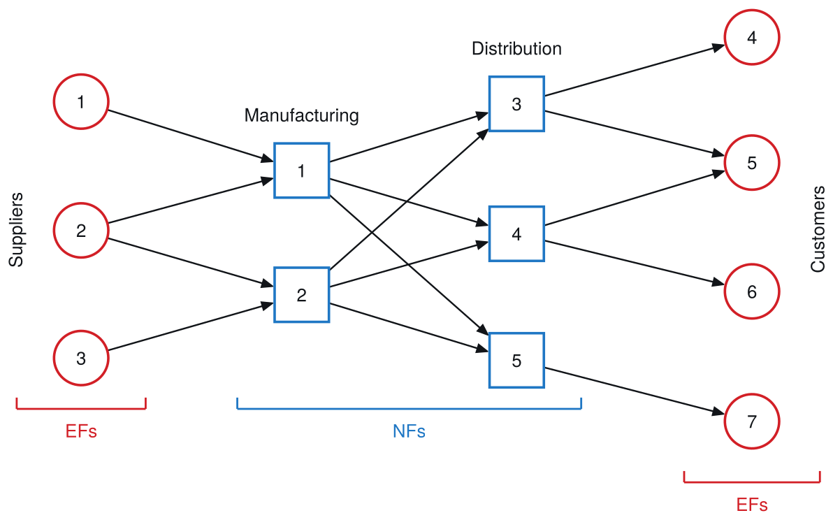
A plus marks a flow the figure draws and a zero marks one it does not, so V and W are the figure written as two tables:
V_{n \times n} = \begin{array}{c|ccccc} \text{NF-NF} & 1 & 2 & 3 & 4 & 5\\ \hline 1 & 0 & 0 & + & + & +\\ 2 & 0 & 0 & + & + & +\\ 3 & 0 & 0 & 0 & 0 & 0\\ 4 & 0 & 0 & 0 & 0 & 0\\ 5 & 0 & 0 & 0 & 0 & 0 \end{array} \qquad W_{n \times m} = \begin{array}{c|ccccccc} \text{NF-EF} & 1 & 2 & 3 & 4 & 5 & 6 & 7\\ \hline 1 & + & + & 0 & 0 & 0 & 0 & 0\\ 2 & 0 & + & + & 0 & 0 & 0 & 0\\ 3 & 0 & 0 & 0 & + & + & 0 & 0\\ 4 & 0 & 0 & 0 & 0 & + & + & 0\\ 5 & 0 & 0 & 0 & 0 & 0 & 0 & + \end{array}
Writing n for the number of new facilities and m for the number of existing ones, with X the n \times d matrix of new-facility locations and P the m \times d matrix of existing ones, the objective is
TC(X) \;=\; \sum_{j=1}^{n}\sum_{k=1}^{n} v_{jk}\, d(X_j, X_k) \;+\; \sum_{j=1}^{n}\sum_{i=1}^{m} w_{ji}\, d(X_j, P_i) \tag{1}
where
- V_{n \times n}
- = NF-NF weights, v_{jk} between new facilities j and k
- W_{n \times m}
- = NF-EF weights, w_{ji} between new facility j and existing facility i
- d
- = number of coordinates a location carries.
Here d = 2, for longitude and latitude. The first double sum is the only new thing, and it is what makes this one problem rather than n of them: move facility j and the cost of every link it has to another new facility moves with it.
It is worth saying plainly how often this general problem gets solved. In thirty or forty years of consulting, never once. It is well developed as theory, and a graduate semester can be spent formulating it as a linear program, but no client has ever asked for manufacturing and distribution to be located together. The manufacturing sites are already there, and the distribution centers are located relative to them. Nor would anyone want them determined together: a plant costs orders of magnitude more than a distribution center, so it is sited on its own terms and the distribution follows.
No interaction between new facilities
Take the manufacturing sites as given and they stop being unknowns: they become two more existing facilities, as in Fig. 3. What is left to locate is the distribution centers, and distribution centers do not ship to one another. Every v_{jk} is therefore zero, the first double sum vanishes, and the objective separates into one term per facility,
TC(X) \;=\; \sum_{j=1}^{n} TC(X_j) \tag{2}
which is a different problem, not merely a smaller one. Three distribution centers in longitude and latitude is a six-dimensional nonlinear optimization while they interact. Separable, it is three two-dimensional problems, each of them the single-facility problem of 2.2. This is the one solved repeatedly, across all kinds of applications.
One thing is assumed away in that figure, and it is the subject of the rest of the lecture: the allocation is drawn as fixed. In practice each customer is served by whichever center turns out nearest, so moving a center changes which customers it serves, and the allocation changes with the location.
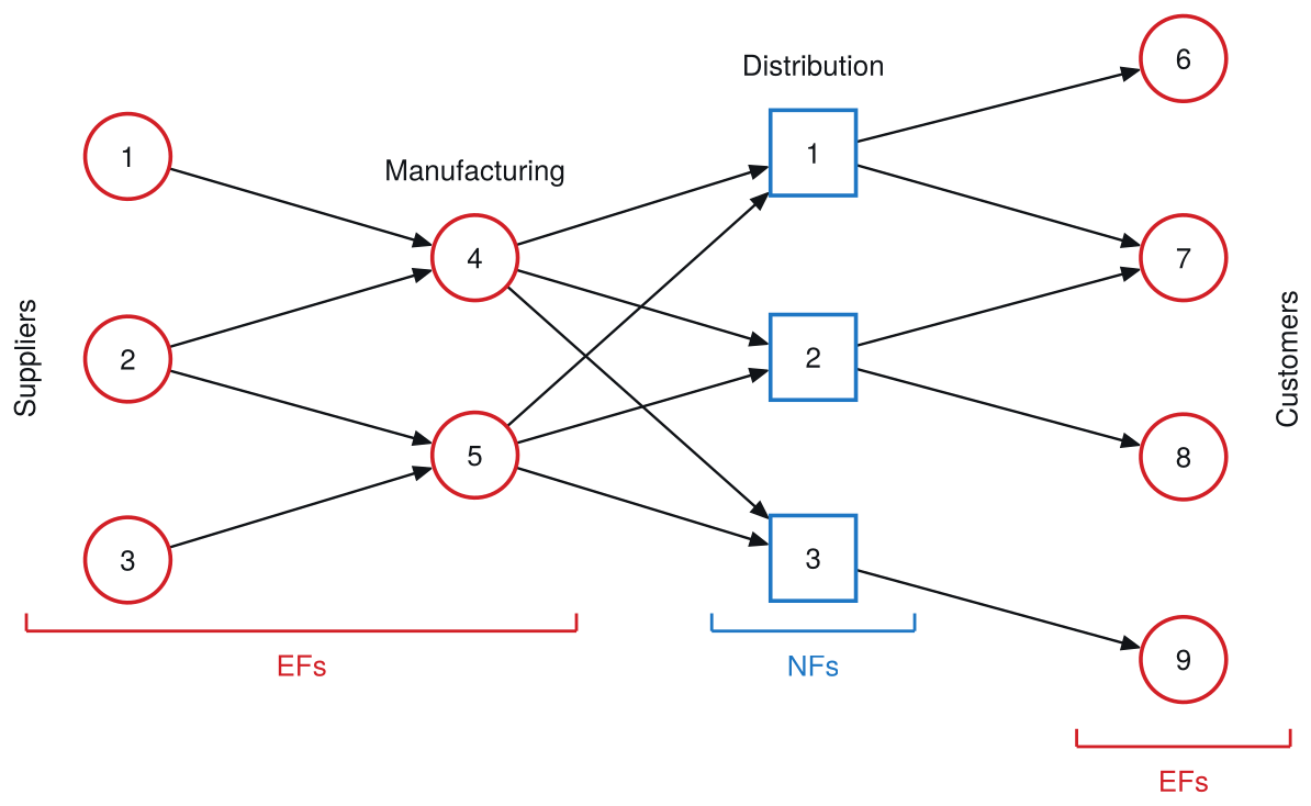
Solving location and allocation together is where Sec. 4 goes. Before that, the interacting case is worth one more look. It is never solved in full, but part of it can be determined without solving anything, and that part answers a question the separable problem cannot even pose.
3. Co-locating operations
Co-location answers the question about how it can be determined where different activities in a supply chain should be co-located, and when it is best to use transportation, when two operations and routing can be split between two locations. The reason this is a problem is that raw materials are typically available at one set of locations, while finished goods are required at a different set of locations, and all of the intermediate processing operations between them can occur either at these locations or at other intermediate locations. This is an important aspect of supply chain design that typically is not discussed in multifacility location, but the majority theorem gives a way of providing an answer.
Theorem
The single-facility form is already familiar from 2.1. If one existing facility carries at least half of all the weight, no search is needed, because the optimum is at that facility:
\text{Locate NF at EF}_j \text{ if } w_j \ge \frac{W}{2}, \quad \text{where } W = \sum_{i=1}^{m} w_i \tag{3}
With several new facilities the same comparison is made row by row, against the weight in both the W and the V matrices, and it does two different things. It can place a facility, as before. It can also co-locate two of them, which is the part with no single-facility analogue: it removes an unknown from the problem without locating it, because instead of having to determine locations for two facilities, only the location for the co-located facilities needs to be determined.
In Model 2 below, the two rules alternate until neither fires, determining which new facilities must share a site and which can be placed at an existing facility, all without computing a single distance.
solve for:
(a) co-located groups among the n NFs;
(b) EF for each group the theorem can place.
subject to:
(a) majority: co-location or placement of a facility is determined only when one weight reaches half of that facility’s own total.
return: placements and co-locations the theorem determines, together with the facilities it leaves open
assumptions:
(a) interactions are symmetric, so the weight between two NFs is the same in either direction;
(b) distance is any metric, since the theorem never evaluates one.
Model 2 formulation: Majority condition
\begin{aligned} \text{co-locate NF } i \text{ and NF } k &\quad \text{if } v_{ik} \ge \gamma_i / 2 \text{ for some } k\\[2pt] \text{place NF } i \text{ at EF } j &\quad \text{if } w_{ij} \ge \gamma_i / 2 \text{ for some } j \end{aligned} \tag{4}
where
- w_{ij}
- = weight between NF i and EF j
- v_{ik}
- = interaction weight between NF i and NF k
- \gamma_i
- = total weight on NF i
- = \sum_{j=1}^{m} w_{ij} + \sum_{k=1}^{n} v_{ik}.
That total runs over both an NF’s customers and its interactions with the other NFs. The two rules are not interchangeable in order. The co-location rule is applied to exhaustion first, each reduction folding two rows into one and so changing the totals the next comparison uses, and only then is the placement rule tried. Ex. 3(c) turns on exactly that: the co-location is what makes the placement possible, and neither facility can be placed before it.
The procedure that applies it is stated at a high level, saying what each pass determines and nothing about how the matrices are kept. Folding one row into another, zeroing a diagonal, turning a placed facility into an existing one: all of that is real, none of it is the idea, and all of it is in the implementation below. Solving using the theorem by hand means applying the rules, not the bookkeeping.
Model 2 formulation: Majority reduction algorithm
algorithm majority;
{ input: NF-to-EF weights W, NF-to-NF weights V }
{ output: settled placements, co-located groups, and what stays open }
begin
done := false;
while done = false do
begin
settled := 0;
for each unsettled NF do
if another NF holds ≥ half of its total weight then
co-locate the two, treat them as one, settled := settled + 1
else if an EF holds ≥ half of its total weight then
place it there, treat it as an EF, settled := settled + 1;
if settled = 0 then done := true;
end;
return the placements, the co-located groups, and what is left open;
end;Two things about it are worth saying before the examples. It is a reduction that sometimes happens to be a solution: it may determine every facility, some of them, or none; and saying which facilities it cannot determine is as much of the answer as saying which it can.
Model 2 implementation: Multifacility majority theorem
function majority(W, V)
W = float(copy(W))
V = float(V == V' ? copy(V) : V + V') # count each once
group = [[i] for i in axes(W, 1)]
at = zeros(Int, size(W, 1))
live, done = collect(axes(W, 1)), false
while !done
done = true
for i in live
γ = sum(W[i, :]) + sum(V[i, :])
k, j = argmax(V[i, :]), argmax(W[i, :])
if V[i, k] > 0 && V[i, k] >= γ / 2 # co-locate
W[i, :] .+= W[k, :]
V[i, :] .+= V[k, :]
V[:, i] .+= V[:, k]
V[i, i] = 0
W[k, :] .= 0; V[k, :] .= 0; V[:, k] .= 0
append!(group[i], group[k]); empty!(group[k])
gone = k
elseif W[i, j] > 0 && W[i, j] >= γ / 2 # place
for r in live # a placed NF becomes an EF
r == i && continue
W[r, j] += V[r, i]
V[r, i] = V[i, r] = 0
end
at[group[i]] .= j
gone = i
else
continue
end
filter!(!=(gone), live); done = false; break
end
end
return at, filter(!isempty, group)
endmajority (generic function with 1 method)Example 3: Limits of the majority theorem
Determine the locations, if any, that the majority theorem determines for two new facilities serving three existing ones, with customer weights W = \begin{bmatrix} 2 & 1 & 0\\ 4 & 0 & 5\end{bmatrix} and a single interaction v between the two, taking v = 2, then v = 0.5, then v = 4.
The same W throughout, and the interaction changed each time. An interaction is given once, in one direction, and is symmetrized before any row is summed:
W = \begin{bmatrix} 2 & 1 & 0\\ 4 & 0 & 5 \end{bmatrix}, \qquad V = \begin{bmatrix} 0 & v\\ 0 & 0 \end{bmatrix} \;\Longrightarrow\; V = \begin{bmatrix} 0 & v\\ v & 0 \end{bmatrix}
Setting the two matrices side by side as [\,W\ \ V\,] turns each facility’s total weight into a single row sum, which is what makes the theorem workable by hand. The dashed rule marks where the customer weights end and the interactions begin, and every comparison below is one row of the augmented matrix against half of its own sum.
Example 3(a): No reduction and no placement
Determine whether the majority theorem reduces or places anything when the flow between the new facilities is v = 2.
With v = 2:
[\,W\ \ V\,] = \left[\begin{array}{ccc:cc} 2 & 1 & 0 & 0 & 2\\ 4 & 0 & 5 & 2 & 0 \end{array}\right] \begin{array}{l} \gamma = 5\\ \gamma = 11 \end{array}
Half of row 1 is 2.5 and its largest entry is 2; half of row 2 is 5.5 and its largest is 5. No entry in either row reaches half of its own row’s total, so the theorem determines nothing at all: no placement, and no co-location.
Example 3(b): Both facilities placed
Determine where both new facilities go when the flow between them is light, v = 0.5.
With v = 0.5:
[\,W\ \ V\,] = \left[\begin{array}{ccc:cc} 2 & 1 & 0 & 0 & 0.5\\ 4 & 0 & 5 & 0.5 & 0 \end{array}\right] \begin{array}{l} \gamma = 3.5 \;\Longrightarrow\; w_{11} = 2 > 1.75 \;\Longrightarrow\; \text{NF1 at EF1}\\ \gamma = 9.5 \;\Longrightarrow\; w_{23} = 5 > 4.75 \;\Longrightarrow\; \text{NF2 at EF3} \end{array}
In both rows the entry that clears sits in W, on the customer side of the rule, so both facilities are placed and the problem is solved outright.
Example 3(c): A reduction, and then a placement
Determine where the new facilities go when the flow between them is heavy, v = 4.
With v = 4:
[\,W\ \ V\,] = \left[\begin{array}{ccc:cc} 2 & 1 & 0 & 0 & 4\\ 4 & 0 & 5 & 4 & 0 \end{array}\right] \begin{array}{l} \gamma = 7 \;\Longrightarrow\; v_{12} = 4 > 3.5 \;\Longrightarrow\; \text{NF1 and NF2 co-located}\\ \gamma = 13 \;\Longrightarrow\; \text{all } w_{ij},\, v_{ij} < 6.5 \end{array}
Row 1 clears on an interaction rather than on a customer, so the two facilities are co-located without either one being placed. Folding them into a single facility adds their customer weights and leaves no interaction behind:
W = \begin{bmatrix} 6 & 1 & 5 \end{bmatrix} \qquad \begin{array}{l} \gamma = 12 \;\Longrightarrow\; w_1 = 6 \ge 6 \;\Longrightarrow\; \text{NF1 (and NF2) at EF1} \end{array}
The reduction did the work the placement rule could not do on its own, which is the half of the theorem with no single-facility analogue.
v = 2: nothing determined. v = 0.5: NF1 at EF1, NF2 at EF3. v = 4: NF1 and NF2 co-located, and the pair at EF1.
Where each operation belongs
The same arithmetic answers the question the section opened with, once the facilities are read as operations rather than buildings. A product passes through a sequence of steps; the first and last are fixed somewhere, and the steps in between could be done anywhere. What the theorem determines is which of them have to share a site.
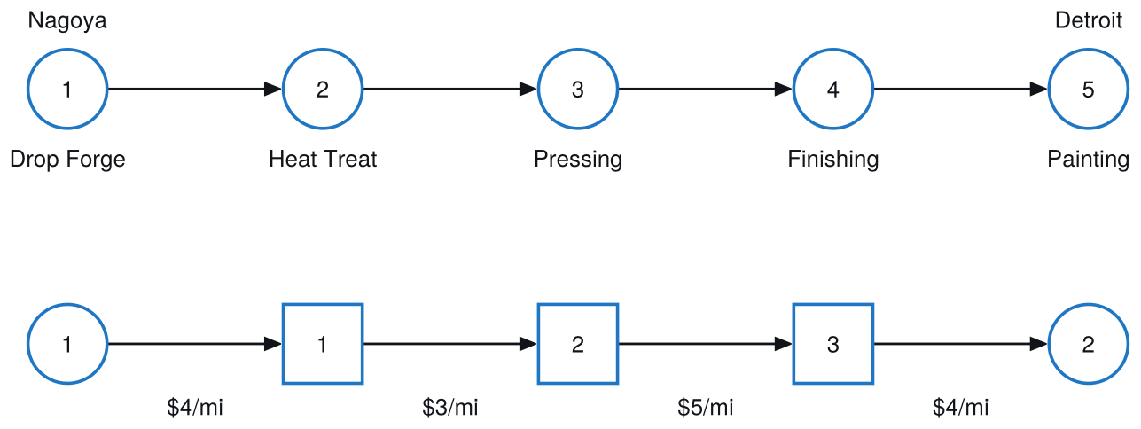
The four rates along the chain in Fig. 4 are not equal, and that is worth a moment before the theorem is applied to them.
The four rates differ. The reason for the difference is that the quantities and characteristics of the materials being moved into an operation in general differ from what comes out of the operation. As a result of the operation, material might be removed, and so the physical weight decreases. Alternatively, materials could be added as part of the operation, and the physical weight would increase. Also, characteristics of the materials could change, resulting in more expensive or cheaper transport alternatives. All of that nets out to differences in transport rates in terms of dollars per mile. This can be seen most clearly by referring back to Eq. 2 in Lecture 2.2, where the monetary weight w_i, in terms of dollars per mile, is the product of the physical weight q_i (tons) and the transport rate r_i ($/ton-mi), both of which can change on the input and output sides of each operation. More details of how to determine these values are discussed in Transport.
Example 4: Five-operation production chain
Determine which of heat treat, pressing and finishing must share a site, and where each of the three operations belongs, given drop forge fixed at Nagoya and painting fixed at Detroit.
Two existing facilities and three new ones. The links to the fixed ends go in W, the links between the three movable operations go in V, and V is symmetrized before any row is summed:
W = \begin{bmatrix} 4 & 0\\ 0 & 0\\ 0 & 4 \end{bmatrix}, \qquad V = \begin{bmatrix} 0 & 3 & 0\\ 0 & 0 & 5\\ 0 & 0 & 0 \end{bmatrix} \;\Longrightarrow\; V = \begin{bmatrix} 0 & 3 & 0\\ 3 & 0 & 5\\ 0 & 5 & 0 \end{bmatrix}
Step 1. One row fires:
[\,W\ \ V\,] = \left[\begin{array}{cc:ccc} 4 & 0 & 0 & 3 & 0\\ 0 & 0 & 3 & 0 & 5\\ 0 & 4 & 0 & 5 & 0 \end{array}\right] \begin{array}{l} \\ \gamma = 8 \;\Longrightarrow\; v_{23} = 5 > 4 \;\Longrightarrow\; \text{NF2 and NF3 co-located}\\ \\ \end{array}
Pressing’s row sums to 8, half is 4, and the 5 it shares with finishing clears it. That is the answer the section asked for: the $5 link between pressing and finishing is expensive enough that moving material along it is not worth doing at all.
Step 2. Fold finishing into pressing, which carries finishing’s link to painting with it:
[\,W\ \ V\,] = \left[\begin{array}{cc:cc} 4 & 0 & 0 & 3\\ 0 & 4 & 3 & 0 \end{array}\right] \begin{array}{l} \gamma = 7 \;\Longrightarrow\; w_{11} = 4 > 3.5 \;\Longrightarrow\; \text{NF1 at EF1}\\ \gamma = 7 \;\Longrightarrow\; w_{22} = 4 > 3.5 \;\Longrightarrow\; \text{NF2 (and NF3) at EF2} \end{array}
Each row’s clearing entry is now a customer weight, so heat treat goes to Nagoya with the drop forge and pressing and finishing go to Detroit with the painting.
Two hand passes determine every operation. majority reaches the same answer without being told which reduction to take first, which is the check worth making once the arithmetic has been done by hand.
operation site
─────────────────────
heat treat Nagoya
pressing Detroit
finishing DetroitPressing and finishing share a site. Heat treat at Nagoya; pressing and finishing at Detroit.
4. Location–allocation problem
The location–allocation (LA) problem is to determine both the location of n new facilities (NFs) and the allocation of the flow requirements of m existing facilities (EFs) to the NFs that minimize total transportation costs.
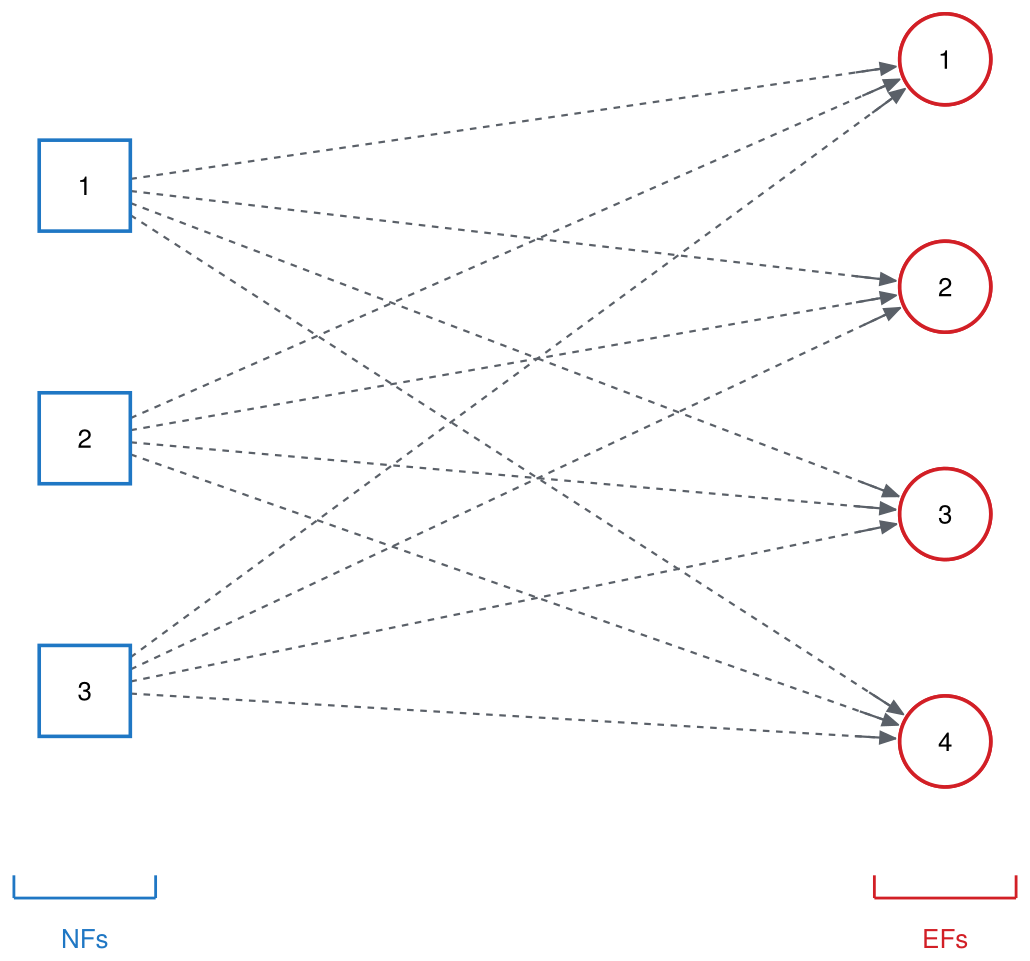
Fig. 5 strips away everything upstream of the NFs, so what is left is the two decisions taken together.
minimize: total transportation cost
solve for:
(a) location of each of the n NFs, anywhere in the plane;
(b) share of each EF’s flow requirement carried by each NF.
subject to:
(a) full allocation: every EF’s flow requirement is allocated in full;
(b) non-negativity: no allocated flow is negative.
return: located NFs together with the allocation that serves the EFs from them
assumptions:
(a) NFs are uncapacitated;
(b) transportation cost is proportional to allocated flow times distance.
Model 3 formulation: Continuous formulation
\begin{aligned} \text{Minimize} \quad & f(X, W) = \sum_{i=1}^{m} \sum_{j=1}^{n} w_{ji} \, d(X_j, P_i) &&\\[2pt] \text{subject to} \quad & \sum_{j=1}^{n} w_{ji} = w_i, && i = 1, \ldots, m \quad (a)\\[2pt] & w_{ji} \ge 0, && j = 1, \ldots, n \quad (b)\\[-2pt] & && i = 1, \ldots, m \end{aligned}
where
- X
- = NF locations
- = [X_j] = [(x_j, y_j)], j = 1, \ldots, n
- W
- = allocated flow requirements
- = [w_{ji}], j = 1, \ldots, n; i = 1, \ldots, m
- P_i
- = location of EF i
- = (a_i, b_i)
- d(X_j, P_i)
- = distance between NF j and EF i
- w_i
- = flow requirement of EF i.
- f(X, W)
- = total transportation cost
- n
- = number of NFs
- m
- = number of EFs.
Two different objects carry the letter w here. The w_{ji} are the elements of the matrix W, one NF’s allocated share of one EF’s requirement, and the w_i are the elements of the vector w, an EF’s requirement in total. The statement is read as an objective function, then a colon, then the constraints to be enforced: each EF’s allocations sum to its requirement, and no allocation is negative. Without that second constraint the problem would be unbounded, since negative weights would let a minimization run off to negative infinity.
Since there are no capacity constraints on the NFs, optimal solutions lie at extreme points of the constraint set of the nonlinear programming (Continuous) formulation of LA problem, i.e., w_{ki} = w_i, for j = k, and w_{ji} = 0, for j \ne k, allocated flow requirements W can be replaced by the allocation vector
\alpha = [\alpha_i], \quad i = 1, \ldots, m, \quad \text{and} \quad \alpha_i \in \{1, \ldots, n\} \tag{5}
resulting in a mixed continuous–combinatorial formulation:
Model 3 formulation: Mixed continuous–combinatorial formulation
\text{Minimize} \quad f(X, \alpha) = \sum_{i=1}^{m} w_i \, d(X_{\alpha_i}, P_i)
If there were constraints on the maximum flow capacity of the NFs, then more than one w_{ji} could be nonzero in an optimal solution and W could not be replaced by the allocation vector \alpha.
NoteSolution space of LA problem
Mix of continuous and combinatorial.
Continuous: X. A 2n-dimensional space of NF locations, X = [(x_1, y_1), \ldots, (x_n, y_n)].
Combinatorial: \alpha.
\left\{ {m \atop n} \right\} = \frac{1}{n!} \sum_{j=1}^{n} (-1)^{n-j} \binom{n}{j} j^m \quad \text{feasible allocations of $n$ NFs to $m$ EFs} \tag{6}
Although n^m allocations are possible, since NFs are indistinguishable, the number of feasible allocations = number of ways m distinguishable EFs can be allocated to n indistinguishable NFs, with each NF allocated to at least one EF = Stirling number of the second kind = \left\{ {m \atop n} \right\}.
For example: \left\{ {7 \atop 2} \right\} = 63, \left\{ {20 \atop 3} \right\} = 5.8 \times 10^8, and \left\{ {65 \atop 5} \right\} = 2.3 \times 10^{43}.
5. Integrated vs alternating
Integrated
If there are no capacity constraints on NFs, it is optimal to always satisfy all the flow requirements of an EF from its closest NF. Requires search of (n \times d)-dimensional TC that combines location with allocation.
Model 3 formulation: Integrated location–allocation formulation
\begin{aligned} \alpha_i(X) &= \arg\min_j \, d(X_j, P_i)\\[2pt] TC(X) &= \sum_{i=1}^{m} w_i \, d(X_{\alpha_i(X)}, P_i)\\[2pt] X^* &= \arg\min_X TC(X)\\[2pt] TC^* &= TC(X^*) \end{aligned}
Alternating
Alternate between finding locations and finding allocations until no further TC improvement. Requires n d-dimensional location searches together with separate allocation procedure. Separating location from allocation allows other types of location and/or allocation procedures to be used:
- Allocation with NF with capacity constraints (solved as minimum cost network flow problem)
- Location with some NFs at fixed locations
Model 3 formulation: Alternating location–allocation formulation
\begin{aligned} allocate(X) &= [w_{ji}] = \begin{cases} w_i, & \text{if } \arg\min_k d(X_k, P_i) = j\\ 0, & \text{otherwise} \end{cases}\\[6pt] TC(X, W) &= \sum_{j=1}^{n} \sum_{i=1}^{m} w_{ji} \, d(X_j, P_i)\\[2pt] locate(W, X) &= \arg\min_X TC(X, W) \end{aligned}
What the objective surface looks like
Both formulations minimize the same total cost, so before choosing between them it is worth seeing the surface either one has to search. A one-dimensional corridor makes that possible to draw: with two facilities on a line, the objective is a function of two numbers and can be contoured in full.
Example 5: Two facilities along I-40
Determine the two mile markers along I-40 that minimize the total weighted distance to the seven cities of Table 1, and show the shape of the objective the search has to work with.
| mile marker | 50 | 150 | 190 | 220 | 270 | 295 | 420 |
| relative demand | 1 | 2 | 3 | 4 | 5 | 6 | 7 |
Interstate 40 crosses North Carolina from the Tennessee line to Wilmington. A city sits at each of seven mile markers, and each city’s weight is its relative demand. Distance along a corridor is rectilinear, so dists is called with p = 1.
50 150 190 220 270 295 420
───────────────────────────────────────
NF 1 50 50 90 120 170 195 320
NF 2 250 150 110 80 30 5 120The integrated formulation folds the allocation into the objective, so the total cost is a function of the locations alone.
TCint (generic function with 1 method)With only two facilities on a line, that objective can be drawn in full (Fig. 6).
Show the code that generates this figure

Starting the search in each basin reaches each optimum.
# Code block 10: two starts, two local optima
Xᵒ¹ = optimize(TCint, [0.0, 200.0]).minimizer
Xᵒ² = optimize(TCint, [200.0, 500.0]).minimizer
prt(DataFrame(start = ["[0, 200]", "[200, 500]"],
NF1 = round.([Xᵒ¹[1], Xᵒ²[1]]; digits = 1),
NF2 = round.([Xᵒ¹[2], Xᵒ²[2]]; digits = 1),
TC = round.([TCint(Xᵒ¹), TCint(Xᵒ²)]; digits = 1))) start NF1 NF2 TC
─────────────────────────────
[0, 200] 190 295 1,340
[200, 500] 270 420 1,050Each axis is one facility’s location, and both span the mile markers along I-40. Two basins appear rather than one, so where the search starts determines which one it ends up in. As the problem gets bigger there are typically more basins to look at, and that is why it is a difficult problem.
Markers 190 and 295 at TC = 1340, or markers 270 and 420 at TC = 1050, according to where the search starts.
6. ALA procedure
Given initial NF locations, ALA local improvement procedure finds optimal EF allocations and then finds optimal NF locations for these allocations, continuing to alternate until no further EF allocation changes are made. Introduced by Cooper in 1963, ALA is still the best heuristic for the LA problem. Since the ALA procedure finds only a local optima, the procedure should be applied multiple times using different initial NF locations, keeping the best solution found as the final solution. This type of repeated application of a local improvement procedure is termed a multistart metaheuristic.
Model 3 formulation: Alternating location–allocation algorithm
algorithm ala;
{ input: starting locations X, weights w, demand points P }
{ output: locations X, allocation W, and total cost TC }
{ allocate is Model 1; locate is the per-facility minisum solve }
begin
W := allocate(X); TC := TC(X, W); done := false;
while done = false do
begin
X′ := locate(W, X);
W′ := allocate(X′);
TC′ := TC(X′, W′);
if TC′ < TC then TC := TC′, X := X′, W := W′
else done := true;
end;
return X, W, TC;
end;Both halves of the loop are already in hand. allocate is Model 1 from Sec. 1, one column of the distance matrix at a time. And in one dimension with rectilinear distance, locate is the median procedure of Model 8 in Lecture 2.1: sort the cities served by a facility, run a cumulative total of their weights, and stop at the city where that total first reaches half. Nothing else is new, which is why the whole procedure can be run on paper.
Example 6: ALA procedure by hand
Determine the locations of two facilities on the I-40 corridor of Ex. 5 by hand, using the ALA procedure from two different pairs of starting locations.
Example 6(a): Starting at mile markers 0 and 200
Determine where the procedure converges from this start, and the total cost there.
Allocate. Facility 1 sits at marker 0 and facility 2 at marker 200, so every city east of marker 100 is nearer facility 2. Only the city at 50 goes to facility 1; the other six go to facility 2.
Locate. Facility 1 serves one city, so it moves to marker 50. Facility 2 serves the cities at 150, 190, 220, 270, 295 and 420, whose weights are 2, 3, 4, 5, 6 and 7 and total 27. Half of that is 13.5. Running west to east, the cumulative weight is 2 at marker 150, 5 at 190, 9 at 220, and 14 at 270, which is the first city at which it reaches 13.5. Facility 2 moves to marker 270.
Three more passes determine it, each one repeating those two steps (Table 2).
| pass | facilities at | facility 1 serves | facility 2 serves | TC | move to |
|---|---|---|---|---|---|
| 1 | 0, 200 | 50 | 150, 190, 220, 270, 295, 420 | 2,720 | 50, 270 |
| 2 | 50, 270 | 50, 150 | 190, 220, 270, 295, 420 | 1,840 | 150, 295 |
| 3 | 150, 295 | 50, 150, 190, 220 | 270, 295, 420 | 1,500 | 190, 295 |
| 4 | 190, 295 | 50, 150, 190, 220 | 270, 295, 420 | 1,340 | 190, 295 |
The fourth pass changes nothing, so the procedure stops at markers 190 and 295 with a total weighted distance of
TC = 1(140) + 2(40) + 3(0) + 4(30) + 5(25) + 6(0) + 7(125) = 1{,}340.
Example 6(b): Starting at mile markers 200 and 500
Determine where the procedure converges from a second start, and whether the two starts agree.
Now facility 1 starts at marker 200 and facility 2 at marker 500, so the midpoint between them is 350 and only the city at 420 lies east of it. Facility 2 takes that city alone and moves to it. Facility 1 takes the other six, whose weights 1 through 6 total 21; half is 10.5, and the cumulative weight running east is 1, 3, 6, 10, then 15 at marker 270, so facility 1 moves there.
| pass | facilities at | facility 1 serves | facility 2 serves | TC | move to |
|---|---|---|---|---|---|
| 1 | 200, 500 | 50, 150, 190, 220, 270, 295 | 420 | 1,840 | 270, 420 |
| 2 | 270, 420 | 50, 150, 190, 220, 270, 295 | 420 | 1,050 | 270, 420 |
The second pass repeats the first pass’s allocation (Table 3), so the procedure stops at markers 270 and 420 with
TC = 1(220) + 2(120) + 3(80) + 4(50) + 5(0) + 6(25) + 7(0) = 1{,}050.
From markers 0 and 200: facilities at 190 and 295, TC = 1340. From markers 200 and 500: facilities at 270 and 420, TC = 1050.
The two runs apply the same procedure to the same seven cities and reach different answers, and the first start reaches the worse of the two. Neither run did anything wrong. That is what a local optimum means here, and it is the reason the procedure is applied from several starts and the best result kept.
The hand work is worth checking, and the check is short because both halves are already written. allocate is Model 1, and the one-dimensional locate is one line: the cumulative weight, and the first city at which it reaches half.
# Code block 11: locate in one dimension, the median of Lecture 2.1
median1(p, wt) = p[findfirst(≥(sum(wt) / 2), cumsum(wt))]
function alatrace(X₀)
X, tr = copy(X₀), DataFrame()
while true
α, TC = allocate(dists(reshape(X, :, 1), P, 1), w)
Xⁿ = [median1(vec(P)[α .== i], w[α .== i])
for i in eachindex(X)]
push!(tr, (at = join(X, ", "), TC = TC,
move = join(Xⁿ, ", ")))
Xⁿ == X && return tr
X = Xⁿ
end
end
prt(alatrace([0, 200]); title = "from markers 0 and 200")
prt(alatrace([200, 500]); title = "from markers 200 and 500")from markers 0 and 200
at TC move
───────────────────────────
0, 200 2,720 50, 270
50, 270 1,840 150, 295
150, 295 1,500 190, 295
190, 295 1,340 190, 295
from markers 200 and 500
at TC move
───────────────────────────
200, 500 1,840 270, 420
270, 420 1,050 270, 420Both traces reproduce Table 2 and Table 3 pass for pass. The same answers come from Logjam.ala, which runs the procedure without any of the scaffolding above, taking the metric as an argument.
Model 3 implementation: Alternating location–allocation algorithm
# Model: Location–allocation, alternating algorithm
# X0: n×2 matrix of initial facility locations (LON, LAT).
# w: length-m vector of demand weights (w_j ≥ 0).
# P: m×2 matrix of demand-point locations (LON, LAT).
# dist: distance metric — :mi (default), :km, :rad (great-circle), or 1/2
# (rectilinear/Euclidean).
# alloc: allocate handle X -> (W, TC) overriding the default
# nearest-facility allocation (e.g. for forced/constrained partitions).
# locate: locate handle (W, X) -> X overriding the default per-facility
# minisum.
# nruns: number of independent random restarts. Run 1 uses X0; runs
# 2…nruns use fresh randX(P, n) starts. The best (minimum-TC) result is
# returned.
ala # (X0, w, P; dist, alloc, locate, nruns) -> (X, TC, W)# Code block 12: the same two starts through ala
Xᵃ, TCᵃ, = ala([0.0; 200.0;;], float(w), float(P); dist = 1)
Xᵇ, TCᵇ, = ala([200.0; 500.0;;], float(w), float(P); dist = 1)
prt(DataFrame(start = ["0, 200", "200, 500"],
NFs = [join(round.(Int, vec(Xᵃ)), ", "),
join(round.(Int, vec(Xᵇ)), ", ")],
TC = round.([TCᵃ, TCᵇ]))) start NFs TC
───────────────────────────
0, 200 190, 295 1,340
200, 500 270, 420 1,050An edge case
What if a NF is not allocated to any EFs? It can happen when the initial NF locations are chosen at random.
North and South Carolina are the example. A bounding box drawn around the cities of those two states covers a large area of the Atlantic, so a randomly chosen starting point can land in the ocean while another lands on the beach. The one on the beach takes the whole allocation and the one at sea is left with nothing. Code could be written to catch that and pick another starting point, but the easier answer is to ignore it and rely on running the procedure from several starts, since one bad start among several does not affect the result kept. Code written for other people to use would handle it properly.
Integrated or alternating
Both only give a local optimal solution (not convex).
The alternating form is more flexible: it solves n d-dimensional location problems with a simple allocation, and Nelder-Mead works well for 2-D. The integrated form solves an (n \times d)-dimensional problem, a larger search, though not a slower one here. Integrated may be better if there are no allocation (e.g., capacity) or location constraints on the NFs.
Running both formulations from the same random starts determines it, provided both are written the same way, from the same allocation step and the same optimizer. On that footing the integrated form is the faster of the two while few facilities are being located, by roughly 1.5 to 2 times at two and three, an advantage that has gone by nine. Quality is close and the lead changes hands: over a common set of starts each form finds the better answer about as often as the other, and the best answers they reach differ by up to 6.5%. So the cost of the choice is in the search, not in the answer.
The advantage of the alternating form is that it provides more flexibility in being able to easily change the allocation and the location mechanisms, so it buys flexibility at the cost of increased computation.
The choice matters less than it might appear, because of the size of the problems actually being solved. A useful rule of thumb is a 10-to-1 ratio: locating ten new facilities calls for a set of about a thousand existing facilities to work with. That is a typical size of problem even for the entire country. Walmart has perhaps 20 or 30 distribution centers, and most large box retailers have 10 to 20, or even around ten.
7. Large-scale examples
Nothing in the procedure changes when the seven cities of the corridor become several hundred places in the plane. What changes is that the answer can no longer be checked by inspection, so the starts have to be generated rather than chosen and the result has to be read back out as a place name.
Two service centers for the Carolinas
Example 7: Service centers for the Carolinas
Determine the two locations that minimize the total population-weighted distance to every city over 10,000 people in North and South Carolina, and the territory each one serves.
155Starting locations are drawn at random from the box around the cities, and ala keeps the best of nruns of them.
idx NAME ST dist bearing dir desc
────────────────────────────────────────────────────────────
8 Charlotte NC 0.0000 3.72 SW in Charlotte, NC
6 Cary NC 0.7437 2.21 SE in Cary, NCDrawing a line from each city to the facility that serves it turns the allocation into a territory (Fig. 7).
Show the code that generates this figure
# Code block 15: mapping the centers and their allocations
Lx, Ly = alloclines(W, Xᵒ, P)
fig, ax = makemap(df.LON, df.LAT; xexpand = 0.1)
for i in eachindex(Lx)
lines!(ax, Lx[i], Ly[i]; linewidth = 0.5)
end
scatter!(ax, Xᵒ[:, 1], Xᵒ[:, 2]; marker = :dtriangle,
markersize = 12, color = :black)
text!(ax, Xᵒ[:, 1], Xᵒ[:, 2]; text = lonlat2loc(Xᵒ, df).NAME,
fontsize = 12, aligntext(Xᵒ[:, 1], Xᵒ[:, 2])...)
fig
Suppose now that a pre-existing contract forces the first three cities to be served by the first facility and the next three by the second. The only thing that changes is the allocation step, which ala accepts as an argument.
# Code block 16: the allocation for a given pair
function alloc36(X)
D = dists(X, P, :mi)
α, = allocate(D, w)
α[1:3] .= 1
α[4:6] .= 2
Wc = sparse(α, 1:nef, w, size(X, 1), nef)
return Wc, sum(Wc .* D)
end
Random.seed!(8345)
Xᶜ, TCᶜ, = ala(randX(P, 2), w, P; alloc = alloc36, nruns = 5)
prt(lonlat2loc(Xᶜ, df)) idx NAME ST dist bearing dir desc
────────────────────────────────────────────────────────────
8 Charlotte NC 0.0000 0.00 N in Charlotte, NC
6 Cary NC 0.0629 2.27 SE in Cary, NCThe same two cities come back, and yet the total is higher: 3.96 against 3.94 hundred million person-miles. That is not an artifact of the random starts. A constraint added to a minimization can never lower the objective, and when it binds it generally raises it. The flexibility the alternating formulation buys is real, but it is paid for in cost.
Service centers at Charlotte and Cary, at 3.94 hundred million person-miles; 0.6% more under the allocation contract.
Best retail warehouse locations
Determining the best retail warehouse locations is an example of a location–allocation problem, where the EFs are population centroids (e.g., ZIP codes). Table 4 lists the best locations for a given number of warehouses. It is assumed that the warehouses serve retail customers located throughout the continental U.S. in proportion to population. Only outbound transport costs are used in making the location decision; it is reasonable to ignore inbound transport as long as suppliers are located uniformly throughout the country so that the inbound transport costs to each warehouse is approximately the same at any location. As can be seen in the table, the best single warehouse location (Bloomington, Indiana) is not the best location as the number of warehouses increases, while the warehouse in Palmdale, California remains in the best west coast location until a second west coast warehouse in Tacoma, Washington is added as part of the five-warehouse solution.
| Number of Locations | Warehouse Location | ||
|---|---|---|---|
| 1 | Bloomington, IN | ||
| 2 | Ashland, KY | Palmdale, CA | |
| 3 | Allentown, PA | Palmdale, CA | McKenzie, TN |
| 4 | Edison, NJ | Palmdale, CA | Chicago, IL |
| Meridian, MS | |||
| 5 | Madison, NJ | Palmdale, CA | Chicago, IL |
| Dallas, TX | Macon, GA | ||
| 6 | Madison, NJ | Pasadena, CA | Chicago, IL |
| Dallas, TX | Macon, GA | Tacoma, WA | |
| 7 | Madison, NJ | Pasadena, CA | Chicago, IL |
| Dallas, TX | Gainesville, GA | Tacoma, WA | |
| Lakeland, FL | |||
| 8 | Madison, NJ | Pasadena, CA | Chicago, IL |
| Dallas, TX | Gainesville, GA | Tacoma, WA | |
| Lakeland, FL | Denver, CO | ||
| 9 | Madison, NJ | Alhambra, CA | Chicago, IL |
| Dallas, TX | Gainesville, GA | Tacoma, WA | |
| Lakeland, FL | Denver, CO | Oakland, CA | |
| 10 | Newark, NJ | Alhambra, CA | Rockford, IL |
| Palistine, TX | Gainesville, GA | Tacoma, WA | |
| Lakeland, FL | Denver, CO | Oakland, CA | |
| Mansfield, OH |
The table is roughly twenty years old, which makes it a test of the method rather than a lookup: the same problem solved against current population data should land in much the same places, and where it does not, the population has moved.
Example 8: Retail warehouse table
Determine the best locations for one, two, three and nine retail warehouses serving the continental United States in proportion to population, and compare them with Table 4.
882The three-digit ZCTA centroids are the existing facilities, about 882 of them, and their populations are the weights. A single warehouse needs no allocation at all, so it is an ordinary single-facility minisum problem. The answer is reported as the nearest city of at least 100,000 people, since a three-digit ZIP code is not a place name.
idx NAME ST dist bearing dir desc
───────────────────────────────────────────────────────────────────────
98 Evansville IN 31.08 6.14 N 31.1 mi N of Evansville, INFrom two warehouses on, the allocation has to be determined with the locations, so ala does the work.
2 warehouses
NAME ST dist
────────────────────────────────────────────
Lexington-Fayette urban county KY 55.42
Visalia CA 106.33
3 warehouses
NAME ST dist
────────────────────────
Visalia CA 94.61
Allentown PA 13.56
Clarksville TN 85.67
9 warehouses
NAME ST dist
──────────────────────────────────────────────────────────────
Mesa AZ 5.40
Chicago IL 2.09
Tacoma WA 53.08
Denver CO 6.10
Waco TX 60.60
Elizabeth NJ 11.11
Lakeland FL 18.72
Santa Clarita CA 9.00
Athens-Clarke County unified government (balance) GA 53.77The map of the nine-warehouse solution shows how the country divides (Fig. 8).
Show the code that generates this figure
# Code block 20: the nine-warehouse allocation
X9 = Xw[9]
W9 = sparse([argmin(c) for c in eachcol(dists(X9, Pz, :mi))],
1:nz, wz, size(X9, 1), nz)
Lx9, Ly9 = alloclines(W9, X9, Pz)
fig9, ax9 = makemap(region = :CUS)
for i in eachindex(Lx9)
lines!(ax9, Lx9[i], Ly9[i]; linewidth = 0.2)
end
scatter!(ax9, X9[:, 1], X9[:, 2]; marker = :dtriangle,
markersize = 10, color = :black)
fig9
None of these points is where a warehouse would actually be built. An optimizer will happily return a swamp, and the site chosen instead is a convenient town near it, along an interstate or better yet at the intersection of two. That substitution is nearly free, because the objective is very flat near its optimum: moving twenty miles to reach a town changes it hardly at all. The town also has to be large enough to staff the place, so five to ten thousand people is a reasonable floor, and towns of that size are usually near an interstate anyway. Those are the practical aspects of it.
One entry in the table is worth a closing note. Not until seven warehouses does one appear in Lakeland, Florida, a town on I-4 about a third of the way from Tampa to Orlando, and it looks like an odd place for it.
It is not an odd place for it. Driving I-4 some years after seeing the table, and passing a sign for Lakeland ten miles ahead, the thought occurred that if the table were true there ought to be distribution centers along here. A minute later there was one under construction, another already built across the road, and over about ten miles two or three dozen of them, warehouses of exactly that massive kind. Somebody was either working from this table or had run the same analysis and reached the same answer.
One warehouse: 31.1 mi N of Evansville, IN. Nine: the table’s Lakeland, Chicago, Tacoma and Denver among them.
Endnotes
Table is adapted from Inbound Logistics, Oct. 2004, p. 50.↩︎