2.7: Discrete Location and MILP

ISE 754: Logistics Engineering, Fall 2026

Data science guides decisions, AI interprets the world—but exponential progress in MILP solvers has had the greater impact on industry, delivering superhuman decision-making for decades.

New Julia packages used

• JuMP is a modeling language for mathematical optimization, embedded in Julia. It lets an optimization problem be written in something close to the notation used on paper, with variables, an objective and constraints declared directly, and then hands that problem to any of a few dozen solvers through one common interface. The same model goes to a different solver by changing one line.
• HiGHS is an open-source solver for linear programs, mixed-integer linear programs and quadratic programs, developed at the University of Edinburgh. It is among the fastest open-source solvers in independent benchmarks, and it is callable from Julia, Python, C++ and the command line.
• Graphs is the standard Julia package for working with graphs: vertices joined by edges, directed or not. It supplies the data structures and the classical algorithms that run on them, such as shortest paths, connectivity, spanning trees and traversals, and it is the base the other graph packages in Julia build on.
• SimpleWeightedGraphs extends Graphs with graph types that carry a weight on every edge, stored as a sparse matrix. It is the type to reach for whenever an edge means a distance, a cost or a capacity rather than merely a connection.
• GraphMakie draws graphs with Makie. It handles the part that is genuinely hard, which is deciding where to put the vertices, and it lets the color, size and label of every vertex and edge be set from data.
• Combinatorics generates and counts the standard combinatorial objects: permutations, combinations, partitions, powersets and their relatives. It is what to reach for when a small instance is to be determined by looking at every possibility.

New Logjam functions used

• snapvals: Snap near-integer and near-zero floating-point values in an array.

Companion script

2-loc-7.jl (PopcoData.csv, PopcoCmatrix.csv, DWTclinics.csv)

1. Introduction to MILP

What computer technology has had the biggest impact on industry since 1990? Data science and analytics; AI, meaning visual and voice recognition, ChatGPT and the rest; or MILP solver improvements?

It is the third, and its biggest impact has been on tactical decisions: production planning and scheduling.

1.1 Math programming

Constraints on the feasibility of a solution can be incorporated into an optimization problem in two ways:

• Penalty methods: the value of the objective function being optimized is somehow degraded at an infeasible solution. The penalties can be either hard or soft, with a soft penalty reducing as a solution gets closer to feasibility.
• Programming methods: the constraints are added to an optimization model as separate functions that are used in the optimization procedure along with the objective function.

A math program is the second of those: an objective function and a set of constraints, stated together and handed to a procedure that respects both. When the objective and every constraint are linear it is a linear program, and Eq. 1 is the one this section works with.

This is the first lecture to take math programming as its subject, but it is not the first to use one. Every model in the course so far has been stated as a callout, with an objective in words, a lettered list of constraints, and a statement of what the model returns, and that format is a math program written in English. The two are worth setting beside each other once. Model 1 is the linear program of Eq. 1 stated the way every model since lecture 1.1 has been stated, and Eq. 1 is the same model in symbols. Lecture 2.1 makes the same crossing in the other direction, from a callout down to the course’s first formulation.

maximize: total value of the two quantities chosen, worth 6 and 8 a unit

solve for:
(a) first quantity, any nonnegative amount;
(b) second quantity, any nonnegative amount.

subject to:
(a) shared supply: the two quantities draw 2 and 3 a unit on a supply of 11;
(b) own supply: first quantity alone draws 2 a unit on a supply of 7.

return: pair of quantities giving the greatest total value

assumptions:
(a) value contributed and supply consumed are proportional to the quantity chosen;
(b) a quantity may be set to any nonnegative real number.

Model 1: Linear program

Model 1 formulation: Linear program

\begin{array}{rlrclll} \textbf{LP} : & \text{Maximize} & 6x_1 + 8x_2 & & & & \\[2pt] & \text{subject to} & 2x_1 + 3x_2 & \leq & 11 & & \\[2pt] & & 2x_1 & \leq & 7 & & \\[2pt] & & x_1,\, x_2 & \geq & 0 & & \end{array} \tag{1}

The correspondence is slot for slot. The objective line becomes the Maximize row. The entries of solve for: become the quantities the operator ranges over, and the values they are allowed to take become the nonnegativity row at the bottom. Each lettered entry of subject to: becomes one constraint row, and the short name it carries is the name that constraint is given when the model reaches JuMP. return: is what the solver reports back.

Two slots do not line up, and both differences are informative. The callout has assumptions:, which bind the data and the world rather than the solution, so they have no row to occupy: a solver is never told them and never checks them, which is why a result has to be checked against them by hand. The program has a where list, which the callout does not, and its appearance is exactly what marks the descent from a model stated as a concept to a model stated as a formulation.

A linear objective is the case where the constraints are not optional. With no limit on x_1 and x_2 the answer is to increase both without bound, since the objective always improves in the same direction; there is no interior point at which it turns over, as there can be for a nonlinear objective. The constraints are what make a finite answer exist at all, and Fig. 1 is the region they leave.

# Two colors carry the section: red is the relaxation and anything
# fractional, green is integer-feasible and what the solver returns.
relaxed  = RGBf(0.78, 0.16, 0.18)
feasible = RGBf(0.13, 0.45, 0.25)
cutline  = RGBf(0.18, 0.40, 0.70)
lattice  = RGBf(0.22, 0.24, 0.27)

c, A, b = (6.0, 8.0), [2.0 3.0; 2.0 0.0], (11.0, 7.0)

function solve_lp(extra = nothing)
    m = Model(HiGHS.Optimizer); set_silent(m)
    @variable(m, x[1:2] >= 0)
    @objective(m, Max, c[1] * x[1] + c[2] * x[2])
    @constraint(m, [k = 1:2], A[k, 1] * x[1] + A[k, 2] * x[2] <= b[k])
    extra === nothing || extra(m, m[:x])
    optimize!(m)
    ok = termination_status(m) == OPTIMAL
    ok || return (obj = NaN, x = [NaN, NaN])
    return (obj = objective_value(m), x = snapvals(value.(x)))
end

lp  = solve_lp()                           # the relaxation
ilp = solve_lp((m, x) -> set_integer.(x))  # the same problem, restricted
inside(i, j) = all(A[k, 1] * i + A[k, 2] * j <= b[k] for k in 1:2)
lat = vec([(i, j) for i in 0:4, j in 0:4 if inside(i, j)])
verts = [(0.0, 0.0), (3.5, 0.0), (3.5, 4 / 3), (0.0, 11 / 3)]

# Each constraint is a line, drawn out to where it meets the axes, so
# the region is visibly their intersection rather than a shape.
x1int = [b[k] / A[k, 1] for k in 1:2]      # where each meets x₂ = 0
x2int = [A[k, 2] == 0 ? Inf : b[k] / A[k, 2] for k in 1:2]

function region_axis(pos, ttl)
    ax = Axis(pos; title = ttl, xlabel = L"x_1", ylabel = L"x_2",
              xticks = 0:6, yticks = 0:4, aspect = DataAspect(),
              titlesize = 17, xlabelsize = 17, ylabelsize = 17,
              xticklabelsize = 15, yticklabelsize = 15)
    limits!(ax, 0, 6.0, 0, 4.2)            # the origin sits in the corner
    for k in 1:2
        isinf(x2int[k]) ?
            lines!(ax, [x1int[k], x1int[k]], [0, 4.2]; color = lattice,
                   linewidth = 1.2, linestyle = :dash) :
            lines!(ax, [0, x1int[k]], [x2int[k], 0]; color = lattice,
                   linewidth = 1.2, linestyle = :dash)
        scatter!(ax, [Point2f(x1int[k], 0)]; color = lattice,
                 markersize = 8, marker = :utriangle)
    end
    poly!(ax, Point2f.(verts); color = (feasible, 0.10),
          strokecolor = feasible, strokewidth = 1.6)
    scatter!(ax, Point2f.(first.(lat), last.(lat)); color = lattice,
             markersize = 7)
    return ax
end

fig = Figure(size = (620, 430))
ax  = region_axis(fig[1, 1],
                  "LP relaxation and the integer points it holds")
text!(ax, 0.12, x2int[1]; text = L"2x_1 + 3x_2 \leq 11", color = lattice,
      align = (:left, :bottom), fontsize = 15)
text!(ax, x1int[2] + 0.08, 4.05; text = L"2x_1 \leq 7", color = lattice,
      align = (:left, :top), fontsize = 15)
scatter!(ax, [Point2f(lp.x...)]; color = relaxed, markersize = 13)
text!(ax, lp.x[1], lp.x[2]; text = @sprintf("  LP optimum  %.2f", lp.obj),
      align = (:left, :center), color = relaxed, fontsize = 15)
scatter!(ax, [Point2f(ilp.x...)]; color = feasible, markersize = 13,
         marker = :diamond)
text!(ax, ilp.x[1], ilp.x[2];
      text = @sprintf("  integer optimum  %.0f", ilp.obj),
      align = (:left, :center), color = feasible, fontsize = 15)
fig

Figure 1: The relaxation, the integer points it holds, and the two optima. Each constraint is drawn out to the axis it meets, so the region is visibly their intersection; the triangles mark where each crosses x_2 = 0. Both objective values are solved for here, not quoted.

Nelder-Mead and gradient-based methods are not reliable procedures for solving problems with a linear objective function. There are specialized procedures like the simplex method (1947) for solving these problems effectively, and the basic idea is as follows:

1. Know, that is, can prove, that the global optimal solution exists at one of the corner points of the feasible region.
2. Pick a starting corner point.
3. If the current corner point is optimal, stop; otherwise
4. Move to an adjacent corner point that improves the objective function and then repeat step 3.

The procedure will eventually terminate at the optimal corner point as long as the feasible region is bounded; otherwise it will report that the problem is unbounded and that no finite optimal solution exists. It will always terminate because, at each corner point considered, the objective is strictly improving. There are also interior point methods that search inside the feasible region; they are often more efficient than the simplex method on large LPs but are less useful when used inside mixed-integer programming solvers.¹

Two packages carry all of this. JuMP provides an algebraic modeling language for creating mathematical programming models, close enough to the notation above that the model can be read off the page; HiGHS is an open-source solver that implements the simplex method, and it is what the models in this course are handed to.

The third rung is the same instance in code. JuMP is a modeling language for Julia: the program is written in it much as it is written on paper, and handed to whichever solver is named.

Model 1 implementation: Linear program

# Model: linear program
using JuMP, HiGHS           # the modeling language, and a solver

m = Model(HiGHS.Optimizer)  # an empty model, and who will solve it
@variable(m, x₁ >= 0)
@variable(m, x₂ >= 0)
@objective(m, Max, 6x₁ + 8x₂)
@constraint(m, 2x₁ + 3x₂ <= 11)
@constraint(m, 2x₁ <= 7)
set_silent(m)               # the solver's own log is not wanted
optimize!(m)
println(termination_status(m))
println("x₁ = ", value(x₁), ", x₂ = ", value(x₂),
        ", obj = ", objective_value(m))

OPTIMAL
x₁ = 3.5, x₂ = 1.3333333333333333, obj = 31.666666666666664

Eight lines, and every one of them is worth naming once, because the rest of this lecture and the whole of the networks topic are written in them.

using JuMP, HiGHS loads two separate things. JuMP is the modeling language and knows nothing about how to solve anything; HiGHS is the solver that does the arithmetic. Keeping them apart is what lets the same model be sent somewhere else by changing one word, which Sec. 1.4 returns to.

Model(HiGHS.Optimizer) creates an empty model and records which solver will be handed it. Everything after that adds to m.

The @ marks a macro, and it is the reason the model reads like the formulation. A macro is handed the expression as text and rewrites it before Julia ever evaluates it, so @constraint(m, 2x₁ + 3x₂ <= 11) can be written the way it appears in Eq. 1. An ordinary function could not: Julia would try to evaluate 2x₁ + 3x₂ <= 11 first, and there is no number in it to compare.

• @variable(m, x₁ >= 0) adds a decision variable and its bounds, written where they would be on paper.
• @objective(m, Max, 6x₁ + 8x₂) takes the sense, Max or Min, and the expression.
• @constraint(m, 2x₁ + 3x₂ <= 11) adds one row.

set_silent(m) turns off the solver’s running commentary, and optimize!(m) sends the model away to be solved. The exclamation mark is Julia’s convention for a function that changes its argument: everything the solver returns is stored back in m, which is why nothing is assigned from it. Afterwards termination_status(m) says whether it solved, objective_value(m) gives the objective, and value(x₁) gives one variable’s value.

The answer is fractional, which is the whole of Sec. 1.2’s problem.

1.2 Integer variables and internal decisions

Mixed-integer programming is used when some of the decision variables need to be integer-valued and/or, more importantly, decisions need to be made as part of the solution procedure, and these “internal decisions” can only be implemented using discrete, typically binary, decision variables. Table 1 is the family, and the name a model takes depends on how much of it is restricted.

Table 1: The four names, and what each restricts.

Name	Short	What it is
Mixed-integer program	MIP	NLP + some integer variables
Mixed-integer linear program	MILP	LP + some integer variables
Integer linear program	ILP	LP + all integer variables
Binary integer program	BIP	LP + all binary variables

Every one of the four is the same generic program with a different restriction laid on it, which Eq. 2 states in one place: the linear program at the top, and below it what each name adds:

\begin{array}{rlrclll} \textbf{LP} : & \text{Maximize} & \mathbf{c}'\mathbf{x} & & & & \\[2pt] & \text{subject to} & \mathbf{A}\mathbf{x} & \leq & \mathbf{b} & & \\[2pt] & & \mathbf{x} & \geq & \mathbf{0} & & \\[8pt] \textbf{MILP} : & \text{some } x_i & & & \text{integer} & & \\[2pt] \textbf{ILP} : & \mathbf{x} & & & \text{integer} & & \\[2pt] \textbf{BIP} : & \mathbf{x} & & & \in \{0, 1\} & & \end{array} \tag{2}

In the following, the focus will be on MILP because it has the widest range of applications. Due to the difficulty in implementing effective procedures, MIP with NLP is usually restricted to only a handful of special NLP models like quadratic programming (QP).

The naming is worth getting straight, because the difficulty follows it. A mixed-integer program is a model with integer variables in it, and the nonlinear kind exists but is rarely tractable. A mixed-integer linear program is the one that recurs: a linear program with some of its variables restricted to the integers. When every variable is so restricted it is an integer linear program, and when every variable is restricted to zero or one it is a binary integer program.

The distinction is made because it buys speed. All-binary is the most tractable, since a solver can exploit what is true of binary variables throughout; all-integer allows some of the same; and a genuine mix of integer and continuous variables is the hardest of the three. Eq. 1 is the linear program the rest of this section restricts.

Restricting x_1 and x_2 of Eq. 1 to the integers leaves only the lattice points of Fig. 1, and the best of them is not the corner the linear program returns. Nor can it be reached by rounding. Just rounding continuous variables to the nearest integer can result in a suboptimal or infeasible solution, and rounding all variables up, or down in a maximization, may be feasible but can result in a poor quality solution. In Eq. 1, rounding the LP solution x_1 = 3.5 to 4 would make the problem infeasible, since the constraint 2x_1 \leq 7 would be violated.

So an integer restriction is not a detail to be tidied up at the end. It is a different problem, and this leads to the three uses of discrete decision variables in a MILP:

1. Integer variable: the variable is inherently discrete. Rounding fails as above. Example: the number of machines, or of trucks.
2. Direct decision: an internal decision variable indicates a choice between two or more alternatives. Binary variables are used, for example, to represent a yes-or-no choice, to indicate or count membership, or to define a relationship, and constraints can then represent logical conditions. Examples: set covering and bin packing, Secs. 3 and 4.
3. Indirect control: an internal decision variable controls other continuous and discrete variables, typically by turning another variable’s lower or upper bound on or off. Taking the product of two variables would be easier to write and would make the model nonlinear, which is the reason for the detour. Examples: the UFL of Sec. 2, where a binary variable decides whether a new facility is located at a site; fixed-charge problems; semi-continuous variables, used to represent a minimum order quantity; a one-time setup cost; and minimum, maximum and absolute values.

The important simplification is that a control variable only has to work when the solver would otherwise want to violate a constraint to improve the solution.

1.3 Branch and bound

For a maximization problem, solving the problem as an LP without integer variable constraints provides an upper bound on the integer-restricted solution. Initially, the lower bound on the solution is zero because the variables are restricted to being nonnegative. Once the first integer feasible solution is found, termed the incumbent solution, it then becomes the current lower bound. The difference between the UB and LB defines the gap, and the search continues through the branch and bound tree until the gap falls below a threshold. Solutions that are not feasible are fathomed, that is, eliminated from the search tree.

Dropping the integer restrictions from a MILP leaves an ordinary linear program, its relaxation. Occasionally the relaxation comes back with every restricted variable already at an integer value, and then there is nothing left to do. Far more often it does not, and the fractional answer is useless as a solution but valuable as a bound. Here it returns x_2 fractional, so it is not a solution to the integer problem, and the gap it opens against a lower bound of zero is about 31. Closing that gap is the whole of what follows: constraints on the variables are added one at a time, forcing them toward integrality, until the gap falls below one. Which of the two openings happens is a property of how the problem was written rather than of integer programming, and Sec. 2.1 is where that turns out to matter: one model in two formulations, one of them tight enough to come back integral at node 0 and the other not.

Example 1: Branch and bound by hand

Determine the integer optimum of the linear program Eq. 1 by adding and dropping constraints on a single model, and confirm it against the same model handed straight to the solver.

Example 1(a): One model, nine nodes

Determine the optimum by solving the relaxation, then adding one constraint at each node and dropping it again when the search moves to the sibling branch, stopping when the gap falls below one.

Before the walk, here is where it arrives. Fig. 2 is the same nine nodes drawn twice: Fig. 2 (a) is the tree the branching builds, each node carrying the two bounds in force when it was reached, and Fig. 2 (b) is where those relaxations land on the feasible region. The blocks that follow produce exactly those nine nodes, one at a time. Read together, the tree is the bookkeeping and the region is what the bookkeeping is about.

# All nine nodes, re-solved here so neither panel can drift from the
# search above. L and G are the two directions a branch can take.
L, G = :le, :ge
paths = Dict(0 => [], 1 => [(1,L,3)], 2 => [(1,L,3),(2,L,1)],
             3 => [(1,L,3),(2,G,2)], 4 => [(1,L,3),(2,G,2),(1,L,2)],
             5 => [(1,L,3),(2,G,2),(1,L,2),(2,L,2)],
             6 => [(1,L,3),(2,G,2),(1,L,2),(2,G,3)],
             7 => [(1,L,3),(2,G,2),(1,G,3)], 8 => [(1,G,4)])
node(cuts) = solve_lp((mm, x) -> for (v, s, r) in cuts
                          s === :le ? @constraint(mm, x[v] <= r) :
                                      @constraint(mm, x[v] >= r)
                      end)
res = Dict(k => node(v) for (k, v) in paths)

function thirds(v)  # 31.667 -> "31 2/3", for a plain string
    w, f = floor(Int, v + 1e-9), v - floor(v + 1e-9)
    f < 1e-6 && return string(w)
    abs(f - 1/3) < 1e-6 && return "$(w)⅓"
    abs(f - 2/3) < 1e-6 && return "$(w)⅔"
    return string(round(v, digits = 2))
end

function texfrac(v)  # 31.667 -> 31\frac{2}{3}, as the slide
    w, f = floor(Int, v + 1e-9), v - floor(v + 1e-9)
    f < 1e-6 && return string(w)
    abs(f - 1/3) < 1e-6 && return string(w) * raw"\frac{1}{3}"
    abs(f - 2/3) < 1e-6 && return string(w) * raw"\frac{2}{3}"
    return string(round(v, digits = 2))
end

# The nodes are visited in order, so the lower bound at each is the best
# integer solution seen up to and including it, and zero before the first.
integral(r) = !isnan(r.obj) && all(r.x .== round.(r.x))  # snapped above
best(id) = [res[j].obj for j in 0:id if integral(res[j])]
lb = Dict(id => maximum([0.0; best(id)]) for id in 0:8)

# The upper bound a node SHOWS is the one still in force: a node that gets
# branched on shows its own relaxation, and a leaf carries its parent's
# down, because nothing better has been solved when the leaf is reached.
par  = Dict(1=>0, 8=>0, 2=>1, 3=>1, 4=>3, 7=>3, 5=>4, 6=>4)
kids = Set(values(par))
ub   = Dict{Int,Float64}()
for id in 0:8
    ub[id] = id in kids ? res[id].obj : ub[par[id]]
end

gx = Dict(0=>0.0, 1=>-1.35, 8=>1.35, 2=>-2.25, 3=>-0.45, 4=>-1.30,
          7=>0.45, 5=>-2.05, 6=>-0.60)
gy = Dict(0=>4.0, 1=>3.0, 8=>3.0, 2=>2.0, 3=>2.0, 4=>1.0, 7=>1.0,
          5=>0.0, 6=>0.0)
blab = Dict(1=>L"x_1 \leq 3", 8=>L"x_1 \geq 4", 2=>L"x_2 \leq 1",
            3=>L"x_2 \geq 2", 4=>L"x_1 \leq 2", 7=>L"x_1 \geq 3",
            5=>L"x_2 \leq 2", 6=>L"x_2 \geq 3")
side = Dict(0=>:right, 1=>:left, 8=>:right, 2=>:left, 3=>:right,
            4=>:left, 7=>:right, 5=>:left, 6=>:right)
incumb = Set([2, 5, 6])  # where a new best integer solution lands

fig = Figure(size = (840, 650))
ax  = Axis(fig[1, 1]; titlesize = 20,
           title = "The bounds close until the gap is under one")
hidedecorations!(ax); hidespines!(ax)
# Wide enough for node 2's caption, and deep enough for the stacked
# fraction in the gap line, which the axis clips if it is not.
limits!(ax, -3.95, 2.75, -1.40, 4.60)

# Centre to centre, and the white-filled circles are drawn over them
# below: the fill hides the overshoot, so every edge meets its node
# exactly, which trimming a fixed amount in y cannot do on an axis
# whose two units are not the same size.
for (kid, pa) in par
    lines!(ax, [Point2f(gx[pa], gy[pa]), Point2f(gx[kid], gy[kid])];
           color = lattice, linewidth = 1.4)
    text!(ax, (gx[pa] + gx[kid]) / 2 + (gx[kid] < gx[pa] ? -0.10 : 0.10),
          (gy[pa] + gy[kid]) / 2 + 0.06; text = blab[kid], fontsize = 20,
          align = (gx[kid] < gx[pa] ? :right : :left, :bottom),
          color = lattice)
end

for id in 0:8
    out = isnan(res[id].obj)
    col = out ? RGBf(0.55, 0.55, 0.58) : id in incumb ? feasible : relaxed
    scatter!(ax, [Point2f(gx[id], gy[id])]; color = :white,
             strokecolor = col, strokewidth = 2.2, markersize = 34)
    text!(ax, gx[id], gy[id]; text = string(id), color = col,
          align = (:center, :center), fontsize = 19)
    dx = side[id] === :left ? -0.30 : 0.30
    al = side[id] === :left ? :right : :left
    if out  # a fathomed node has no bounds to show
        text!(ax, gx[id] + dx, gy[id]; text = "fathomed,\ninfeasible",
              align = (al, :center), color = col, fontsize = 17)
        continue
    end
    u, l = texfrac(ub[id]), texfrac(lb[id])
    dy = id in incumb ? 0.13 : 0.0
    text!(ax, gx[id] + dx, gy[id] + dy; text = L"UB = %$u, \; LB = %$l",
          align = (al, :center), color = lattice, fontsize = 20)
    id in incumb &&
        text!(ax, gx[id] + dx, gy[id] - 0.22; text = "incumbent",
              align = (al, :center), color = feasible, fontsize = 17)
end
text!(ax, gx[0] + 0.30, gy[0] + 0.30; text = "LP", color = relaxed,
      align = (:left, :center), fontsize = 19, font = :bold)

g6, l6 = texfrac(ub[6]), texfrac(lb[6])
text!(ax, -0.85, -0.70; align = (:right, :top), color = lattice,
      fontsize = 20, text = L"gap = %$g6 - %$l6 < 1 \; \Rightarrow")
text!(ax, -0.78, -0.70; align = (:left, :top), color = feasible,
      fontsize = 19, font = :bold, text = "stop")
fig
off = Dict(0 => (0.10, -0.16), 1 => (0.10, 0.10), 2 => (0.10, -0.14),
           3 => (0.10, 0.10), 4 => (-0.12, 0.12), 5 => (-0.12, -0.16),
           6 => (0.10, 0.10))

fig = Figure(size = (620, 450))
ax  = region_axis(fig[1, 1], "Every node is an LP over a smaller region")
for id in 0:6
    q = res[id].x
    scatter!(ax, [Point2f(q...)]; color = relaxed, markersize = 11)
    text!(ax, q[1] + off[id][1], q[2] + off[id][2];
          text = L"%$id: \; %$(texfrac(res[id].obj))",
          align = (:left, :center), color = relaxed, fontsize = 17)
end
scatter!(ax, [Point2f(ilp.x...)]; color = feasible, markersize = 14,
         marker = :diamond)
fig

(a) The tree. Each node carries the upper bound in force when it was evaluated and the best integer solution found so far, and the constraint that created it is on the edge above.

(b) The same nodes on the feasible region, each at the point its own relaxation returned and labeled with that node’s objective. Nodes 7 and 8 are infeasible and have no point to plot.

Figure 2: The search twice over, the tree above and the region below.

First, solve as an LP, which is branch node 0 in the tree. Every node after it is the same model: a node adds a constraint, and moving to a sibling drops it again. Nothing else changes, and that is the whole of the method.

# Code block 1: one node's report, printed the same way every time
function prtnode(m, UB, LB, x₁, x₂)
    xᵒ = snapvals(value.([x₁, x₂]))
    println("Obj: ", objective_value(m),
            ", x₁: ", xᵒ[1], ", x₂: ", xᵒ[2])
    println(" UB: ", UB, ", LB: ", LB, ", Gap: ", UB - LB, "\n")
    return nothing
end

prtnode (generic function with 1 method)

# Code block 2: node 0, the relaxation
m = Model(HiGHS.Optimizer)
@variable(m, 0 <= x₁)  # continuous, for now
@variable(m, 0 <= x₂)
@objective(m, Max, 6x₁ + 8x₂)
@constraint(m, 2x₁ + 3x₂ <= 11)
@constraint(m, 2x₁ <= 7)
set_silent(m)
optimize!(m)
println(termination_status(m))
UB, LB = objective_value(m), 0.0
prtnode(m, UB, LB, x₁, x₂)

OPTIMAL
Obj: 31.666666666666664, x₁: 3.5, x₂: 1.3333333333333333
 UB: 31.666666666666664, LB: 0.0, Gap: 31.666666666666664

Next, select one of the fractional decision variables and add two integer constraints to the tree: x_1 \leq 3 on one side and x_1 \geq 4 on the other. Selection of the variable can be based on the most fractional, the least fractional, and many other criteria.

One piece of syntax is new here. A constraint may be given a name, the c1 in @constraint(m, c1, x₁ <= 3), and the name is how it is referred to again: delete(m, c1) removes it from the model, which is how the search crosses from a branch to its sibling below.

# Code block 3: node 1, adding x₁ ≤ 3
@constraint(m, c1, x₁ <= 3)
optimize!(m)
println(termination_status(m))
UB = objective_value(m)
prtnode(m, UB, LB, x₁, x₂)

OPTIMAL
Obj: 31.333333333333336, x₁: 3.0, x₂: 1.6666666666666667
 UB: 31.333333333333336, LB: 0.0, Gap: 31.333333333333336

# Code block 4: node 2, adding x₂ ≤ 1, the first incumbent
@constraint(m, c2, x₂ <= 1)
optimize!(m)
println(termination_status(m))
LB = objective_value(m)
prtnode(m, UB, LB, x₁, x₂)

OPTIMAL
Obj: 26.0, x₁: 3.0, x₂: 1.0
 UB: 31.333333333333336, LB: 26.0, Gap: 5.333333333333336

Both variables are integer, so this is a feasible solution to the original problem: the incumbent, and the first real lower bound. The search now crosses to the sibling branch, which means dropping the constraint that defined this one.

# Code block 5: node 3, dropping x₂ ≤ 1 and adding x₂ ≥ 2
delete(m, c2)
@constraint(m, c3, x₂ >= 2)
optimize!(m)
println(termination_status(m))
UB = objective_value(m)
prtnode(m, UB, LB, x₁, x₂)

OPTIMAL
Obj: 31.0, x₁: 2.5, x₂: 2.0
 UB: 31.0, LB: 26.0, Gap: 5.0

# Code block 6: node 4, adding x₁ ≤ 2
@constraint(m, c4, x₁ <= 2)
optimize!(m)
println(termination_status(m))
UB = objective_value(m)
prtnode(m, UB, LB, x₁, x₂)

OPTIMAL
Obj: 30.666666666666668, x₁: 2.0, x₂: 2.3333333333333335
 UB: 30.666666666666668, LB: 26.0, Gap: 4.666666666666668

# Code block 7: node 5, adding x₂ ≤ 2, a better incumbent
@constraint(m, c5, x₂ <= 2)
optimize!(m)
println(termination_status(m))
LB = objective_value(m)
prtnode(m, UB, LB, x₁, x₂)

OPTIMAL
Obj: 28.0, x₁: 2.0, x₂: 2.0
 UB: 30.666666666666668, LB: 28.0, Gap: 2.666666666666668

# Code block 8: node 6, dropping x₂ ≤ 2 and adding x₂ ≥ 3
delete(m, c5)
@constraint(m, c6, x₂ >= 3)
optimize!(m)
println(termination_status(m))
LB = objective_value(m)
prtnode(m, UB, LB, x₁, x₂)

OPTIMAL
Obj: 30.0, x₁: 1.0, x₂: 3.0
 UB: 30.666666666666668, LB: 30.0, Gap: 0.6666666666666679

At node 6, the absolute value of the gap was less than one, and as a result, the procedure could stop. In practice, only the relative percentage gap is determined, and the search continues until the gap approaches zero or the complete tree has been searched; as a result, in practice, nodes 7 and 8 might be evaluated before being fathomed. Since the branch and bound tree can grow exponentially, in many applications the search can be stopped when the relative gap falls below a value of 1%, for example.

# Code block 9: node 7, infeasible and therefore fathomed
delete(m, [c4, c6])
@constraint(m, c7, x₁ >= 3)
optimize!(m)
termination_status(m)

INFEASIBLE::TerminationStatusCode = 2

# Code block 10: node 8, infeasible, and the tree is now searched
delete(m, [c1, c3, c7])
@constraint(m, c8, x₁ >= 4)
optimize!(m)
termination_status(m)

INFEASIBLE::TerminationStatusCode = 2

Nine nodes, one model, and every bound in Fig. 2 (a) printed along the way.

Example 1(b): The same problem handed straight to the solver

Determine the same optimum by declaring the variables integer and letting the solver run its own branch and bound.

During the solution of large MILP models, such as those used for production-inventory planning, small rounding errors accumulate. The function snapvals(v) is used in place of Array(value.(v)) to set any solution value to an integer if it is close to an integer. A variable declared binary can come back as 0.9999999997, which is not 1 to any test that asks whether it is, and every solution read in this lecture goes through snapvals for that reason.

# Code block 11: the integer program, declared and solved in one step
m = Model(HiGHS.Optimizer)
@variable(m, 0 <= y₁, Int)       # integer variable
@variable(m, 0 <= y₂, Int)
@objective(m, Max, 6y₁ + 8y₂)
@constraint(m, 2y₁ + 3y₂ <= 11)
@constraint(m, 2y₁ <= 7)
set_silent(m)
optimize!(m)
yᵒ = snapvals(value.([y₁, y₂]))  # no near-integers in the answer
println("Obj: ", objective_value(m), ", y₁: ", yᵒ[1], ", y₂: ", yᵒ[2])

Obj: 30.0, y₁: 1.0, y₂: 3.0

x_1 = 1, x_2 = 3, with an objective of 30

One thing in that model is new, and it is the only thing. Int at the end of a @variable line restricts that variable to the integers, and Bin restricts it to zero or one; everything else is Model 1’s implementation rung unchanged. Nine nodes of branching became one word.

The same answer, and the interesting part is what it cost. A solver can be asked to show its work, and on a problem this size it has to be asked twice: with the default settings its presolve and its heuristics land on the answer before any branching, so there is no search to watch. Switching presolve off and turning the heuristic effort down to zero leaves one.

# Code block 12: make the solver branch, and show what it does
b = Model(HiGHS.Optimizer)           # the same model again
@variable(b, 0 <= z₁, Int)
@variable(b, 0 <= z₂, Int)
@objective(b, Max, 6z₁ + 8z₂)
@constraint(b, 2z₁ + 3z₂ <= 11)
@constraint(b, 2z₁ <= 7)
set_attribute(b, "presolve", "off")  # no shortcut to the answer
set_attribute(b, "mip_heuristic_effort", 0.0)
optimize!(b)                         # not silent: print the log

Running HiGHS 1.15.1 (git hash: 04024d701f): Copyright (c) 2026 under MIT licence terms
Includes third-party software components, see THIRD_PARTY_NOTICES.md for full details
Using BLAS: libblastrampoline 
MIP has 2 rows; 2 cols; 3 nonzeros; 2 integer variables (0 binary)
Coefficient ranges:
  Matrix  [2e+00, 3e+00]
  Cost    [6e+00, 8e+00]
  Bound   [0e+00, 0e+00]
  RHS     [7e+00, 1e+01]

Presolve is switched off
Objective function is integral with scale 0.5

Solving MIP model with:
   2 rows
   2 cols (0 binary, 2 integer, 0 implied int., 0 continuous, 0 domain fixed)
   3 nonzeros
   Thread count 16 (of 32 threads). Using 1 max workers. Parallel search off

Src: B => Branching; C => Central rounding; F => Feasibility pump; H => Heuristic;
     I => Shifting; J => Feasibility jump; L => Sub-MIP; P => Empty MIP; R => Randomized rounding;
     S => Solve LP; T => Evaluate node; U => Unbounded; X => User solution; Y => HiGHS solution;
     Z => ZI Round; l => Trivial lower; p => Trivial point; u => Trivial upper; z => Trivial zero

        Nodes      |    B&B Tree     |            Objective Bounds              |  Dynamic Constraints |       Work      
Src  Proc. InQueue |  Leaves   Expl. | BestBound       BestSol              Gap |   Cuts   InLp Confl. | LpIters     Time

 z       0       0         0   0.00%   inf             -0                 Large        0      0      0         0     0.0s
 J       0       0         0   0.00%   inf             24                 Large        0      0      0         0     0.0s
 S       0       0         0   0.00%   42              26                61.54%        0      0      0         0     0.0s
 S       0       0         0   0.00%   31.33333333     28                11.90%        0      0      1         0     0.0s
 T       0       0         0   0.00%   30.66666667     30                 2.22%        1      1      1         1     0.0s
         1       0         1 100.00%   30              30                 0.00%        1      1      1         1     0.0s

Solving report
  Status            Optimal
  Primal bound      30
  Dual bound        30
  Gap               0% (tolerance: 0.01%)
  P-D integral      0.000143969379211
  Solution status   feasible
                    30 (objective)
                    0 (bound viol.)
                    2.22044604925e-16 (int. viol.)
                    0 (row viol.)
  Timing            0.01
                    0.00 (Presolve)
                    0.01 (Solve)
                    0.00 (Postsolve)
  Max sub-MIP depth 0
  Nodes             1
  Repair LPs        0
  LP iterations     1
                    0 (strong br.)
                    1 (separation)
                    0 (heuristics)

The table in the middle of that output is the same search, run by the solver. BestBound is the upper bound and BestSol is the incumbent, so the two columns are the UB and LB of Fig. 2 (a), and Gap is the distance between them. Read down: the bound falls from 42 to 31⅓ to 30⅔ to 30 while the incumbent climbs from 24 to 26 to 28 to 30, and the last three of each are the numbers the nine nodes produced by hand. The Src column says what produced each row, decoded by the legend printed above it: S is an LP solve, T an evaluated node, J a heuristic that jumps to a feasible point, and B a branching. The first two rows have an infinite bound because no LP has been solved yet, which is the same state the nine nodes start in, with a lower bound of zero.

In general none of this is wanted. set_silent is the normal setting, as it is on every other model in this lecture: the result is what matters and a real model’s log runs to thousands of lines. The two attributes above exist only to make a search visible on a problem too small to need one, and the model was declared a second time because re-solving the first would have handed the solver its own previous answer to start from, which is again no search at all.

Two settings do matter on a model that is not small, and both appear later in the course. A time limit, set_time_limit_sec(m, 60.0), stops the search and returns the best solution found so far, with termination_status reporting TIME_LIMIT rather than OPTIMAL, and Sec. 4’s bin packing is where it earns its keep. A gap tolerance stops it earlier on purpose: as Sec. 1.3 says, in many applications the search is stopped when the relative gap falls below one percent, and relative_gap(m) is what that is measured against. A MILP that returns at the time limit has still returned something usable, which is the practical difference between it and an LP.

1.4 MILP solvers

A solver does a great deal more than the nine nodes of Ex. 1. It removes variables it can prove are fixed before the search starts, it adds cuts that remove fractional vertices without removing any integer point, it runs heuristics to find an incumbent early so the lower bound is not zero for long, and in parallel it uses the separate cores of the machine to solve nodes in the B&B tree.²

Presolve is the cheapest of those and the easiest to see. From 2x_1 + 2x_2 \leq 1 with x_1, x_2 \geq 0 and integer, it follows that x_1 = x_2 = 0, so both variables and the constraint can be removed before the search starts.

Over 2001 to 2020 the machines got about 20 times faster and the algorithms about 50 times better, which is roughly a thousandfold together.³ That is a large number, and it is much smaller than what came before it: the growth did not extend far past 2000, and the largest single step was taken in the 1990s. What was taken then was a backlog. Some thirty years of theory on cutting planes and on presolve had been published and left unimplemented, and one release of one solver put as much of it into code as its authors could manage.⁴⁵

Where the step change came from is worth knowing, because it is not the kind of thing that happens twice. CPLEX was the first commercial solver and for most of the 1980s it had the market to itself, which is a position with no reason in it to make the product faster. Meanwhile the published theory on cutting planes and on presolve had been accumulating, largely unimplemented, for some thirty years: work a commercial code could have taken up at any time and had not.

Robert Bixby is the one who eventually spent it, and he had co-founded CPLEX himself. He and two colleagues went through that literature, took the theoretical advances no commercial code had picked up, and implemented as many of them as they could; the work took months rather than years, and one release came out of it more than ten times faster than the one before. Once it was done the other vendors followed.⁶

That is the mechanism behind the figures above, and it is also the reason to expect the curve to bend. A backlog of unimplemented theory can be cleared once.

The figures for the earlier window are larger and they are a different study. From 1990 to 2014, for MILP solvers, computer speed accounts for about 320,200\times and algorithm improvements for about 580,000\times, which together turn ten days of round-the-clock processing in 1990 into one second in 2014. Since 2014 the speed-up has slowed, to something on the order of 5 to 15\times, and solver development has gone into other things.⁷

Reading the two windows together is what makes the point sharper rather than weaker. Single-thread hardware gains flattened through the 2010s while algorithmic gains did not, so the claim that algorithm improvement has outrun computer speed over the period is more true now than when it was first made.⁸

Table 2 is the field a model is handed to. JuMP supports many more than these;⁹ what the table gives is the few that are met in practice.

Table 2: The commercial and open-source MIP solvers most often met.

Solver	Kind	Note
CPLEX	Commercial	IBM, first commercial solver
Gurobi	Commercial	Developed by Robert Bixby (best commercial)
FICO Xpress	Commercial	Used by Coupa
SAS/OR	Commercial	Part of SAS system (not supported in JuMP)
HiGHS	Open-source	Originated at University of Edinburgh (best open-source)
Cbc	Open-source	COIN-OR solver
GLPK	Open-source	Free Software Foundation GNU solver (legacy)

Moving a model from one of them to another costs one line. The only differences in JuMP when using different solvers are which optimizer the model is built with, Model(HiGHS.Optimizer) against Model(Gurobi.Optimizer), and the names of any solver-specific attributes that are set. Nothing about the model itself changes, which is the reason for writing it in a modeling language rather than against one solver’s own interface.

A cut is the part of that worth seeing, and Fig. 3 is one. It is a constraint the integer problem already satisfies and the relaxation does not, so adding it removes fractional territory and no integer point at all. The classic way to produce one is the Gomory cut, read off the simplex tableau of the relaxation itself, which is what makes cutting a thing a solver can do unaided: it needs nothing but the LP it has just solved.

cut_rhs = 4.0  # x₁ + x₂ ≤ 4, through (1,3) and (3,1)

@assert all(i + j <= cut_rhs + 1e-9 for (i, j) in lat)  # valid
@assert sum(lp.x) > cut_rhs + 1e-9                      # and it cuts

fig = Figure(size = (620, 430))
ax  = region_axis(fig[1, 1],
      "A cut removes the fractional vertex, not an integer point")
lines!(ax, [Point2f(0, cut_rhs), Point2f(cut_rhs, 0)]; color = cutline,
       linewidth = 2, linestyle = :dash)
text!(ax, 4.15, 0.35; text = L"x_1 + x_2 \leq 4", color = cutline,
      fontsize = 16)
scatter!(ax, [Point2f(lp.x...)]; color = relaxed, markersize = 13)
text!(ax, lp.x[1], lp.x[2]; text = "  cut off", align = (:left, :center),
      color = relaxed, fontsize = 15)
fig

Figure 3: A valid cut removes the fractional vertex and no integer point. The line drawn is the facet of the integer hull through the two best integer points, rather than any particular Gomory cut, and both properties that make it a cut are asserted in the code rather than taken by eye.

2. Discrete facility location as a MILP

The UFL is where a mixed-integer program is worth meeting for the first time, and for two reasons. It is a problem already understood well enough to check a model against something: lecture 2.4 solved this same problem by heuristic, so there is an answer to compare with. And the formulation buys a capability no heuristic in that lecture has, which is that a constraint can simply be added to it. What comes later, network flow and production-inventory systems, is much harder to hold in the head, and arriving there already fluent in a MILP is worth the detour.

One more property makes the UFL a forgiving place to start. Under the strong formulation of Eq. 4 the relaxation at node 0 is very often integral already, and then the optimum arrives with no branching at all. That is the exception Sec. 1.3 promised rather than a contradiction of it: a relaxation is usually fractional, and this one usually is not, because Eq. 4 is written tightly enough to make it so.

Only part of what a facility costs bears on where it goes. Total production cost is a line in the quantity produced, an intercept plus a rate, and lecture 2.6 fits it to obtain both. The rate is charged per ton wherever the plant stands, so it is the same whatever the answer is and drops out of the comparison. What is left is the intercept, which is incurred once per facility built, and the transport cost, which is the part that depends on where the facility is. Those two together are the total logistics cost of Eq. 3, and they are what the models in this section minimize:

\begin{array}{lrcl} \text{Total production cost:} & TPC & = & k + c_p f \\ \text{Total transport cost:} & TC & = & f r d \\ \text{Total logistics cost:} & TLC & = & k + f r d \end{array} \tag{3}

where

k

= fixed production cost, in dollars per year

c_p

= unit production cost, in dollars per ton

f

= production rate, in tons per year

r

= transport rate, in dollars per ton-mile

d

= transport distance, in miles.

2.1 Uncapacitated facility location

The set-notation statement of the problem is lecture 2.4’s, and it is not restated here: Model 1 in Lecture 2.4 is the concept and its mathematical formulation rung carries the Y^{\star} that this lecture works from. Read it as a sentence: determine the set of sites Y that minimizes the fixed cost of opening them plus the cost of serving every existing facility from the site it is assigned to, subject to every existing facility being served. The bars around Y^{\star} count the elements of the set rather than taking an absolute value, so the number of facilities opened is read off the answer rather than fixed in advance.

The single constraint is what forces the assignment to be complete. Without it the cheapest thing to do is open nothing and serve no one, since every cost in the objective is incurred only by doing something.

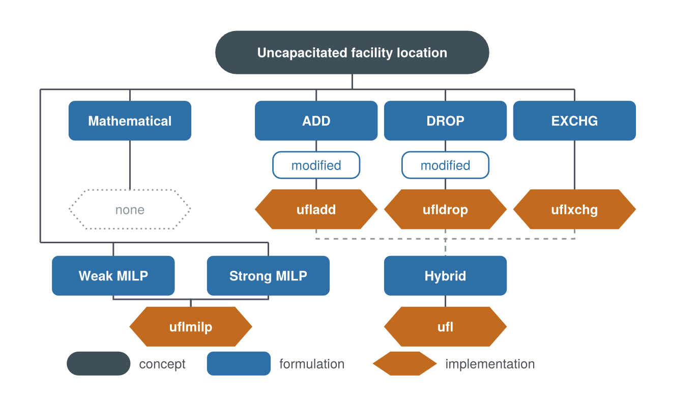
Being uncapacitated allows simple heuristics to be used to solve the UFL, and Fig. 4 is the map of them: ADD construction adds one NF at a time, DROP construction drops one at a time, XCHG improvement moves one NF at a time to unoccupied sites, and the HYBRID algorithm combines ADD and DROP construction with XCHG improvement, repeating until no change in Y. HYBRID is the default heuristic for the UFL and it is what lecture 2.4 uses.¹⁰ What this lecture adds is the branch on the left, and it is the first time the mathematical side of that tree has reached a runnable implementation.

Figure 4: The resolution rungs of Model 1 in Lecture 2.4, with the MILP branch this lecture adds. Lecture 2.4 built the mathematical formulation and the four heuristic formulations, each heuristic carrying a Logjam implementation and the mathematical one carrying none. The two MILP formulations of Secs. 2.1 and 2.2 share one implementation, which is the JuMP model a solver is handed.

Lecture 2.4 states the UFL in set notation and this section states it as a math program. The two say the same thing, and they are not equally useful. The set form is the one that suggests a heuristic, because it is written in terms of which existing facilities a site serves. The math program suggests only that a solver be called, and a reader meeting the problem for the first time in this form would conclude that a MILP is the only way to solve it. A great many published papers do exactly that: they open with a formulation, for a problem a heuristic would have handled well.

minimize: total of facility fixed cost and transport cost

solve for:
(a) sites at which to locate new facilities, a subset of the n candidate sites.

subject to:
(a) coverage: every existing facility is fully served;
(b) linking: nothing is served from a site unless a facility is established there.

return: sites chosen and the resulting total cost

assumptions:
(a) new facilities may be located only at the given candidate sites;
(b) new facilities are uncapacitated, so every existing facility is served by whichever open site is cheapest.

Model 2: Uncapacitated facility location

Model 2 is Model 1 in Lecture 2.4 restated, word for word, and it is here because the rungs below hang from it. Nothing about the concept changes when the method does, which is the whole point of the device: what follows is the same decision resolved a different way.

Model 2 formulation: MILP formulation

\begin{array}{rlrclll} & \text{Minimize} & \displaystyle \sum_{i \in N} k_i y_i + \sum_{i \in N}\sum_{j \in M} c_{ij} x_{ij} & & & & \\[2pt] & \text{subject to} & \displaystyle \sum_{i \in N} x_{ij} & = & 1, & j \in M & (a) \\[2pt] & & y_i & \geq & x_{ij}, & i \in N,\; j \in M & (b) \\[2pt] & & 0 \leq x_{ij} & \leq & 1, & i \in N,\; j \in M & \\[2pt] & & y_i & \in & \{0,1\}, & i \in N & \end{array} \tag{4}

where

k_i

= fixed cost of an NF at site i \in N = \{1, \ldots, n\}

c_{ij}

= variable cost from site i to serve EF j \in M = \{1, \ldots, m\}

y_i

= \begin{cases} 1, & \text{if an NF is established at site } i \\ 0, & \text{otherwise} \end{cases}

x_{ij}

= fraction of EF j’s demand served from the NF at site i.

The UFL problem is a MILP because the y_i’s are binary variables and the x_{ij}’s are real variables. In the UFL problem, all x_{ij} are 0 or 1; in the capacitated facility location (CFL) problem of Sec. 2.2, there is a maximum capacity associated with each site, resulting in an x_{ij} value between 0 and 1 whenever not all of an EF j’s demand can be served from the NF at site i.

Two constraints carry the model. The first requires every existing facility to be fully assigned: the fractions serving it sum to one. The second is what forces a site to be opened before anything can be served from it, and it is the constraint that makes the fixed cost unavoidable. Without it nothing would ever open, since the objective is a minimization and a site that serves no one costs nothing.

The allocation variables are declared continuous on the unit interval rather than binary. In the UFL they come back 0 or 1 without being told to, so nothing is bought by forcing them, and the only variables that have to be restricted are the y_i: one establishes a site, zero does not.

Constraint (b) is one per site-and-facility pair, nm of them, each saying that a site must be open before that one existing facility is served from it. Written that way it is the strong formulation, and its relaxation typically returns the optimum outright.

There is a looser way to say the same thing, and it is worth knowing because it was once the default. The nm constraints can be collapsed to n, one per site, by capping the whole of what a site serves at m, the largest number of existing facilities any one site could take. That is the weak formulation of Eq. 5: true, and loose, so its relaxation stops well short of the optimum and leaves a large tree for branch and bound.

Model 2 formulation: Weak MILP formulation

Constraint (b) alone is replaced, and the symbols are those above:

\begin{array}{rlrclll} & & m\,y_i & \geq & \displaystyle \sum_{j \in M} x_{ij}, & i \in N & (b) \end{array} \tag{5}

The reason to reach for it is memory, and only memory: nm constraints can exhaust it on a large instance where n of them fit. Machines now have enough that this is much less often the binding thing than it used to be, so the strong form is the sensible default and the weak one is what is written when the strong one will not fit. Both say that a site must be open before anything is served from it, so the concept above them does not change; what changes is how much of the work is left to the solver, which is what the rungs are for.

Model 2 implementation: Uncapacitated facility location

# Model: uncapacitated facility location, the strong formulation
function uflmilp(k, C)
    n, m = size(C)
    N, M = 1:n, 1:m
    u = Model(HiGHS.Optimizer)
    set_silent(u)
    @variable(u, y[N], Bin)                  # open a site, or not
    @variable(u, 0 <= x[N, M] <= 1)          # share of EF j served from i
    @objective(u, Min, sum(k[i] * y[i] for i in N) +
                       sum(C[i, j] * x[i, j] for i in N, j in M))
    @constraint(u, coverage[j in M],         # (a)
                sum(x[i, j] for i in N) == 1)
    @constraint(u, linking[i in N, j in M],  # (b)
                y[i] >= x[i, j])
    optimize!(u)
    yᵒ = snapvals(value.(y))
    res = (Y = findall(==(1.0), yᵒ), X = snapvals(value.(x)),
           TC = objective_value(u))
    return res
end

uflmilp (generic function with 1 method)

The implementation is Eq. 4 and nothing else: y is binary, the linking constraints are the nm of the strong form, and there is no switch to throw. A model written for a reader is written one way. Eq. 5 is a change of one constraint if a particular instance ever needs it.

Example 2: Five I-40 cities as a MILP

Determine the sites and the total cost for the five cities of lecture 2.4, which are Asheville, Statesville, Greensboro, Raleigh and Wilmington, at mile markers 50, 150, 220, 295 and 420 along I-40, each with unit demand and costing 150, 200, 150, 150 and 200 to establish, and determine whether the answer its heuristics reached is the best one.

# Code block 13: the five I-40 cities of lecture 2.4, through the model
P = [50 150 220 295 420]'          # mile markers along I-40
r, f = 1, 1                    # rate and flow, both unit here
w = r * f
k = [150, 200, 150, 150, 200]  # fixed cost of a site
C = w * dists(P, P, 1)         # variable cost, site to customer
strg = uflmilp(k, C)
# uflmilp returns X through snapvals, so these are exact 0s and 1s
prt(DataFrame(Site = strg.Y,
              Serves = [string(findall(==(1), strg.X[i, :]))
                        for i in strg.Y]))

  Site     Serves
─────────────────
     1     [1, 2]
     4  [3, 4, 5]

Sites 1 and 4 at TC = 600

That is the same pair of sites, and the same total cost, that the hybrid heuristic of lecture 2.4 reached on this data by a wholly different route, and the agreement of two independent procedures is a Triangulate check on both.

It is also more than that, and the more is what this section is for. Lecture 2.4 could say that its heuristics had stopped improving; it could not say that nothing better existed, because a heuristic has no way to know. The MILP does: branch and bound terminates by proving that the bound and the incumbent have met, so 600 is not merely the best answer found but the best answer there is.

Example 3: Popco’s plants to optimality

Determine the optimal set of bottling plants for the Popco instance of lecture 2.6, and determine how much the heuristic used there left on the table.

The instance is 2.6’s. Its step 5 builds the cost matrix over 204 candidate sites and 162 customers, saved here rather than rebuilt, and its step 1 regresses the fixed cost out of what the 42 plants spend on production.

# Code block 14: Popco's cost matrix and fixed cost, from lecture 2.6
DC = DataFrame(CSV.File("data/PopcoData.csv"))
CP = Matrix(DataFrame(CSV.File("data/PopcoCmatrix.csv")))
kP = ([ones(nrow(DC)) DC.DEMAND] \ DC.PROD_COST)[1]  # the intercept
(k = round(kP), sites = size(CP, 1), customers = size(CP, 2))

(k = 1.0603652e7, sites = 204, customers = 162)

# Code block 15: the same rung, at 204 sites
popco = uflmilp(fill(kP, size(CP, 1)), CP)
(plants = length(popco.Y), TC = round(popco.TC))

(plants = 24, TC = 7.2547914e8)

24 plants at a total cost of $725.5M a year, and this one is optimal

Compare the MILP solution with the heuristic solution of lecture 2.6: which is “better”?

# Code block 16: the optimum against the heuristic, on the same data
yh, TCufl, Wh = ufl(kP, CP)  # the heuristic of lecture 2.6
above = round(100 * (TCufl - popco.TC) / popco.TC, digits = 3)
prt(DataFrame(Case = ["heuristic", "MILP"],
              Plants = [length(yh), length(popco.Y)],
              TC = round.([TCufl, popco.TC]),
              Above = ["$above%", "-"]))

  Add: 7.512802717682018e8
 Xchg: 7.27809919688256e8
  Add: 7.27809919688256e8
 Drop: 7.260353153560858e8
 Xchg: 7.260353153560858e8
       Case  Plants           TC   Above
────────────────────────────────────────
  heuristic      24  726,035,315  0.077%
       MILP      24  725,479,140       -

The two answers are worth putting side by side before either is trusted. The MILP is optimal and the heuristic is not, and the distance between them is a small fraction of one percent. Against that, the data underneath is nowhere near so accurate: the rate was backed out of a single year’s spending, the customers are ZIP-code centroids standing in for the real ones, and one intercept is charged at every candidate site. A gap of that size is comfortably inside the margin of error of the inputs, which is the honest way to ask what the MILP was for.

It was not for the saving. What it establishes is the quality of the heuristic: across the instances this course has run, the heuristics of lecture 2.4 have never come back worse than about three percent, and here they land within a tenth of one. Knowing that costs one solve, and it is what makes the heuristic usable on the problems where no solver will finish.

The comparison doubles as a Bounds check on the MILP. The heuristic’s answer is feasible for the same model, so the optimum cannot cost more than it does. A solver returning a larger number would be reporting a defect in how the model was written rather than an answer to it.

2.2 Capacitated facility location

Model 3 is the same decision under a capacity, and Eq. 6 changes one line of Eq. 5 to get there. Constraint (b) becomes a capacity constraint: what a site serves is the demand of the existing facilities allocated to it, \sum_{j \in M} f_j x_{ij}, and that cannot exceed K_i when the site is open, nor be anything but zero when it is not. Everything else stands as it was. The capacity is data, and handing it to the model is the whole of the change.

minimize: total of facility fixed cost and transport cost

solve for:
(a) sites at which to locate new facilities, a subset of the n candidate sites;
(b) share of each existing facility’s demand served from each open site.

subject to:
(a) coverage: every existing facility’s demand is fully served;
(b) capacity: no new facility is asked for more than it can produce.

return: sites chosen, the allocation, and the resulting total cost

assumptions:
(a) new facilities may be located only at the given candidate sites;
(b) each candidate site has a stated capacity.

Model 3: Capacitated facility location

Model 3 formulation: Capacitated facility location

\begin{array}{rlrclll} & \text{Minimize} & \displaystyle \sum_{i \in N} k_i y_i + \sum_{i \in N}\sum_{j \in M} c_{ij} x_{ij} & & & & \\[2pt] & \text{subject to} & \displaystyle \sum_{i \in N} x_{ij} & = & 1, & j \in M & (a) \\[2pt] & & K_i\,y_i & \geq & \displaystyle \sum_{j \in M} f_j x_{ij}, & i \in N & (b) \\[2pt] & & 0 \leq x_{ij} & \leq & 1, & i \in N,\; j \in M & \\[2pt] & & y_i & \in & \{0,1\}, & i \in N & \end{array} \tag{6}

where the symbols of Eq. 5 carry over, and

K_i

= capacity of an NF at site i \in N, in tons per year

f_j

= demand of EF j \in M, in tons per year.

The capacity constraint replaces the linking constraint rather than joining it, which is the compact thing about this model and is easy to miss: K_i y_i does the work of m y_i, so a site with nothing allocated to it is forced closed by the same line that caps an open one.

One consequence belongs here, because it is an Assumptions check on the model just above. Under a capacity the allocations x_{ij} can come back genuinely fractional, an existing facility split between two sites, so the argument for declaring them continuous in Eq. 5 no longer holds as a statement about the answer. It holds as a modeling choice, and whether a split allocation is acceptable is a question about the situation rather than about the solver.

Two more of these cost a line each, and they belong beside the capacity.

When the number of NFs is specified and all of the fixed costs are identical, or not stated, then the fixed costs will have no impact on the location decision and can be set to zero in the objective, and the following constraint can be added to the UFL problem to formulate the p-median problem:

\sum_{i \in N} y_i = p \tag{7}

where p is the number of NFs to be located and Eq. 7 is the only line added. If non-identical fixed costs are included, then the p-median problem generalizes to the p-UFL problem, where both are special cases of it.

A new facility at a given site is simpler still: y_i = 1 fixes it open and y_i = 0 rules it out. In JuMP neither needs a constraint, since a variable can be fixed in place with fix(y[3], 1; force = true), and the solver then optimizes around it. That is how an incumbent plant that cannot be closed, or a site already bought, enters the analysis.

What the three have in common is the point of the section. Each is a line of algebra against a model that already exists, and none of them is available to a heuristic that works by choosing a set of sites and assigning each customer to the nearest open one.

A site that can produce only so much takes one more constraint: whatever is served from it must not exceed its capacity. That is the whole of the capacitated problem, and it is the clearest illustration of what the formulation buys. None of the heuristics in lecture 2.4 can be pointed at it. They choose a set of sites and let each existing facility go to its nearest open one; there is nowhere in that procedure to put a limit on how much any one site absorbs. The MILP takes the limit as a line of algebra.

Model 3 implementation: Capacitated facility location

# Model: capacitated facility location
function cflmilp(k, C, f, K)
    n, m = size(C)
    N, M = 1:n, 1:m
    c = Model(HiGHS.Optimizer)
    set_silent(c)
    @variable(c, y[N], Bin)
    @variable(c, 0 <= x[N, M] <= 1)
    @objective(c, Min, sum(k[i] * y[i] for i in N) +
                       sum(C[i, j] * x[i, j] for i in N, j in M))
    @constraint(c, coverage[j in M],  # (a) coverage
                sum(x[i, j] for i in N) == 1)
    @constraint(c, capacity[i in N],  # (b) capacity
                K[i] * y[i] >= sum(f[j] * x[i, j] for j in M))
    optimize!(c)
    yᵒ = snapvals(value.(y))
    res = (Y = findall(==(1.0), yᵒ), X = snapvals(value.(x)),
           TC = objective_value(c))
    return res
end

cflmilp (generic function with 1 method)

Example 4: Capacitated EMCA

Determine how many machines EMCA should lease and where to locate them with each machine’s capacity accounted for, on the instance of lecture 2.4: twelve million units a year sold to customers grouped by the twenty-eight three-digit ZIP codes of the Carolinas, each unit weighing 15 pounds and shipped at $0.25 per ton-mile, each machine leased for $100,000 per year and able to produce up to two million units a year.

This is the example lecture 2.4 left open. The heuristics there have nowhere to put a capacity, so what that lecture did instead was raise the number of machines until no machine was over its limit, and it closed by saying the capacity would be handled once this lecture had covered it. The data is 2.4’s, unchanged.

One thing is not 2.4’s, and it has to be determined before the model is given a capacity. A machine that can make two million units a year cannot be planned to make two million: lecture 1.3 has cycle time running away as utilization approaches one, which is why 2.4 rejects six machines for this instance, saying that six would carry “a utilization of exactly one, and a workstation is designed to run with its utilization strictly below one”.

So the capacity the model is handed is an effective capacity, the nameplate times a ceiling on utilization, and the ceiling comes from lecture 1.3 rather than from nowhere. Its feasible minimum m_{\min} = \lfloor r_a t_e + 1 \rfloor is the rule that forces the utilization below one by adding a machine, and the utilization it implies here is 6/7.

# Code block 17: EMCA's customers, as lecture 2.4 sets them up
zips = [
    270, 271, 272, 273, 274, 275, 276, 277, 278, 279, 280, 281, 282, 283,
    284, 285, 286, 287, 290, 291, 292, 293, 294, 295, 296, 297, 298, 299]
nc = [
      7,   5,   6,   3,   5,   8,   5,   1,   3,   2,   8,   4,   9,   6,
      1,   2,   3,   3,   4,   3,   3,   2,  11,   5,   7,   2,   4,   2]
ud, uwt = 12e6, 15 / 2000                   # units/yr in total, ton/unit
units = ud .* nc ./ sum(nc)                 # units/yr by ZIP
fz = units .* uwt                           # ton/yr by ZIP
zc = uszcta3()
iz = [findfirst(==(zi), zc.ZCTA3) for zi in zips]
Pz = hcat(zc.LON[iz], zc.LAT[iz])           # ZIP centroids
Cz = (fz .* 0.25)' .* (1.2 .* dists(Pz, Pz, :mi))    # $/yr, circuity 1.2
kz = fill(100_000.0, length(zips))          # $/yr per machine
K = 2e6                                     # units/yr a machine CAN make
mmin = floor(Int, ud / K + 1)  # lecture 1.3's feasible minimum
umax = (ud / K) / mmin                      # the utilization it plans to
Kmach = fill(umax * K * uwt, length(zips))  # ton/yr, effective
(sites = length(zips), mmin = mmin, umax = round(umax, digits = 3))

(sites = 28, mmin = 7, umax = 0.857)

# Code block 18: the same decision with the capacity in the model
cfl = cflmilp(kz, Cz, fz, Kmach)
cflraw = cflmilp(kz, Cz, fz, fill(K * uwt, length(zips)))  # no ceiling
made = vec(sum(cfl.X .* fz', dims = 2))     # ton/yr at each site
prt(DataFrame(ZIP = zips[cfl.Y], tons = round.(made[cfl.Y]),
              util = round.(made[cfl.Y] ./ (K * uwt),      # of NAMEPLATE
                            digits = 3)))

   ZIP    tons    util
──────────────────────
1  270  12,857  0.8570
2  272  11,302  0.7530
3  275  12,857  0.8570
4  282  12,857  0.8570
5  283  10,369  0.6910
6  290  11,613  0.7740
7  294   9,435  0.6290
8  296   8,710  0.5810

8 machines at a total annual cost of $1,346,321

Code block 19 puts that beside the four other answers this instance has, and the spread is the point of the section. The arithmetic floor is twelve million units over two million a machine, and it is not achievable: it is the utilization of one that lecture 1.3 rules out, which is why the feasible minimum sits a machine above it. The UFL opens the floor’s six anyway and is no solution at all, its busiest machine asked for more than a machine can make. Lecture 2.4’s sweep is feasible and expensive: with no way to put the capacity into the heuristic it buys feasibility with machines. The CFL puts the capacity where it belongs and lands one machine above 1.3’s minimum.

# Code block 19: four answers to the same question
yu, TCu, Wu = ufl(kz[1], Cz; verbose = false)  # no capacity
su = vec(sum(Wu .* units', dims = 2))[yu]
nm, over, TCh, sh = mmin, true, 0.0, Float64[]
while over                                     # lecture 2.4's sweep
    global nm, over, TCh, sh
    yh, TCp, W = pmedian(nm, Cz; verbose = false)
    sh = vec(sum(W .* units', dims = 2))[yh]
    TCh = TCp + nm * kz[1]
    over = maximum(sh) > K
    over && (nm += 1)
end
busiest(s) = 100 * maximum(s) / K              # % of NAMEPLATE capacity
ans = DataFrame(
    approach = ["floor: units / capacity", "throughput-feasible minimum",
                "UFL, capacity ignored", "sweep on the heuristic",
                "CFL as a MILP"],
    machines = [ceil(Int, ud / K), mmin, length(yu), nm, length(cfl.Y)],
    pct = round.([100.0, 100 * umax, busiest(su), busiest(sh),
                  100 * maximum(made[cfl.Y]) / (K * uwt)], digits = 1),
    TC = round.([NaN, NaN, TCu, TCh, cfl.TC]))
prt(ans)

                     approach  machines     pct         TC
──────────────────────────────────────────────────────────
      floor: units / capacity         6  100.00           
  throughput-feasible minimum         7   85.70           
        UFL, capacity ignored         6  135.50  1,248,233
       sweep on the heuristic        17   72.60  1,796,918
                CFL as a MILP         8   85.70  1,346,321

Two readings are worth taking from that table rather than one. The machine count is the visible saving, 9 fewer, but the cost is the one that matters: the MILP’s answer is 25% cheaper than the sweep’s, and the saving is smaller than the machine count makes it look. The 9 machines the MILP does not lease are worth $900,000 a year on their own, but 8 machines stand further from the demand than 17 do, so $449,402 of that goes straight back into transport cost, and the $450,598 left over is what the percentage reports.

The pct column says it a second way, and it is read against the nameplate rather than against the effective capacity the model was given. The sweep stops as soon as its busiest machine is inside the nameplate, and by then that machine is running at 73% of it, so the seventeen are not seventeen full machines. The MILP runs its busiest at 86%, which is the ceiling it was planned to and is strictly below one, as 1.3 requires.

The ceiling costs almost nothing here, and that is worth knowing rather than assuming. Planned to the nameplate the same model opens the same eight machines at $1,301,411, so the whole of what the ceiling buys is 3% on the bill and no extra machine. It is below 0.85 that the count starts to rise.

A second reading is an Assumptions check, and it is the one this section warned about. 2 of the twenty-eight ZIP codes come back split across two machines, which is the fractional x_{ij} that a capacity makes possible. Whether a customer group can be served from two machines is a question about EMCA rather than about the solver, and if the answer is no then the x_{ij} have to be declared binary and the model re-solved.

3. Set covering and set packing

The set covering problem refers to minimizing the number of sets whose union includes all of the objects to be covered. Each set can include (or cover) a different subset of objects, and multiple sets can cover each. There are many applications of set covering; for example, each set might represent the customers that are within a one-hour drive of a potential site for a service center, and a solution to the set covering problem would correspond to the minimum number of sites required so that each customer can be serviced within one hour.

minimize: total cost of the subsets chosen

solve for:
(a) subsets to include in the cover.

subject to:
(a) coverage: every object belongs to at least one chosen subset.

return: subsets chosen and the resulting cost

assumptions:
(a) subsets are given;
(b) overlap is permitted, so an object may be covered more than once.

Model 4: Set covering

Model 4 is the model, and it is resolved twice. The set-theoretic statement of Eq. 8 comes first, and the order is deliberate: it is the form a heuristic can be read out of, where the binary program below it is the form a solver can be handed.

Model 4 formulation: Mathematical formulation

\begin{array}{rcl} M & = & \{1, \ldots, m\}, \quad \text{objects to be covered} \\ M_i \subseteq M,\; i \in N & = & \{1, \ldots, n\}, \quad \text{subsets of } M \\ c_i & = & \text{cost of using } M_i \text{ in cover} \\ I^{\star} & = & \displaystyle\arg\min_{I}\Bigl\{ \sum_{i \in I} c_i \;:\; \bigcup_{i \in I} M_i = M \Bigr\} \\ & & \text{min cost covering of } M \end{array} \tag{8}

Model 4 formulation: Math-programming formulation

\begin{array}{rlrclll} & \text{Minimize} & \displaystyle \sum_{i \in N} c_i x_i & & & & \\[2pt] & \text{subject to} & \displaystyle \sum_{i \in N} a_{ji} x_i & \geq & 1, & j \in M & (a) \\[2pt] & & x_i & \in & \{0,1\}, & i \in N & \end{array} \tag{9}

where

x_i

= \begin{cases} 1, & \text{if } M_i \text{ is in the cover} \\ 0, & \text{otherwise} \end{cases}

a_{ji}

= \begin{cases} 1, & \text{if } j \in M_i \\ 0, & \text{otherwise} \end{cases}.

Fig. 5 is six objects and five subsets drawn, which is the instance Ex. 5 works. An object inside two enclosures is in both subsets, and a covering is allowed to use it twice.

Figure 5: Six objects, and the five subsets available to cover them. Where two enclosures overlap the object inside belongs to both, which is what a covering permits and what makes the matrix \mathbf{A} of Eq. 9 more than a list.

Unweighted is the usual case, c_i = 1 for every subset, and then the objective counts subsets. The implementation takes the whole instance as the one matrix \mathbf{A} = [\,a_{ji}\,], since that is the only thing that changes from one application to the next. It prints its termination status, because the messaging is otherwise off and there would be nothing to say whether an optimal solution was found.

Model 4 implementation: Set covering

# Model: set covering, given any object-by-subset matrix
function setcover(A)
    M, N = 1:size(A, 1), 1:size(A, 2)
    model = Model(HiGHS.Optimizer)
    @variable(model, x[1:length(N)], Bin)
    @objective(model, Min, sum(x[i] for i in N))
    @constraint(model, coverage[j in M],  # (a)
                sum(A[j, i] * x[i] for i in N) >= 1)
    set_silent(model)
    set_time_limit_sec(model, 60.0)       # solution timeout
    optimize!(model)
    println(solution_summary(model).termination_status)
    return findall(==(1.0), snapvals(value.(x)))
end

setcover (generic function with 1 method)

Good heuristics for covering exist, and they are rarely needed. The relaxation of Eq. 9 is tight enough that very large instances solve outright, which makes this one of the easy problems for a MILP solver and one of the few places in this course where reaching for the solver first is the right instinct.

The application that recurs is a service radius, and the one this course meets again in Topic 3 is the road network. Select the minimum number of intersections, that is nodes, such that every intersection in the network is within a stated distance of one of the selected ones. The selected intersections could be locations for truck terminals, and the coverage distance represents the maximum a truck can travel in one day to reach the others. The radius is what defines the subsets, so changing it is the whole of the sensitivity analysis.

The set packing problem differs from the set covering problem in its treatment of overlap. In a covering, an object may appear in more than one of the selected subsets, since the goal is simply to ensure that every object is included in at least one chosen set. In a packing, by contrast, no object may appear in more than one selected subset, overlap is forbidden, and consequently some objects may remain uncovered. In terms of the binary integer programming formulation, the objective in a packing problem is to maximize the number of subsets selected, whereas in a covering problem the objective is to minimize the number of subsets required to achieve full coverage. Model 5 is that problem, and Eq. 10 is one character from Eq. 9.

maximize: number of subsets chosen

solve for:
(a) subsets to include in the packing.

subject to:
(a) disjointness: no object belongs to more than one chosen subset.

return: subsets chosen, and the objects left uncovered

assumptions:
(a) subsets are given;
(b) not every object need be covered.

Model 5: Set packing

Model 5 formulation: Set packing

\begin{array}{rlrclll} & \text{Maximize} & \displaystyle \sum_{i \in N} x_i & & & & \\[2pt] & \text{subject to} & \displaystyle \sum_{i \in N} a_{ji} x_i & \leq & 1, & j \in M & (a) \\[2pt] & & x_i & \in & \{0,1\}, & i \in N & \end{array} \tag{10}

where the symbols of Eq. 9 carry over.

Set packing is the mirror of covering rather than a problem in its own right: it asks for the most subsets that can be chosen with no object in two of them, where covering asks for the fewest that leave no object in none. It is carried here for the contrast, and a use for it has yet to come up in practice.

Model 5 implementation: Set packing

# Model: set packing, which is set covering with two characters changed
function setpack(A)
    M, N = 1:size(A, 1), 1:size(A, 2)
    model = Model(HiGHS.Optimizer)
    @variable(model, x[N], Bin)
    @objective(model, Max, sum(x[i] for i in N))
    @constraint(model, disjoint[j in M],  # (a)
                sum(A[j, i] * x[i] for i in N) <= 1)
    set_silent(model)
    optimize!(model)
    return findall(==(1.0), snapvals(value.(x)))
end

setpack (generic function with 1 method)

Fig. 6 is the packing of the same six objects Fig. 5 covers, and reading the two together is the quickest way to see the difference the two characters make. The subsets it leaves out are drawn dashed, because each of them overlaps one that was taken.

Figure 6: The largest packing of the same six objects. No object lies in two chosen subsets, and object 4, ringed in red, lies in none, which a packing permits and a covering forbids. The dashed subsets are the ones left out: each overlaps one that was taken.

3 subsets in the packing, I^{\star} = {1, 3, 5}, leaving object 4 uncovered

Example 5: Six objects and five subsets

Determine the smallest collection of the five subsets whose union is all six objects, where the subsets are M_1 = \{1,2\}, M_2 = \{1,4,5\}, M_3 = \{3,5\}, M_4 = \{2,3,6\} and M_5 = \{6\}, each costing the same.

Fig. 5, drawn above, is this instance. Mi holds the five subsets it draws, and the model wants them as the matrix \mathbf{A} instead.

# Code block 20: the five subsets as an object-by-subset matrix
m, n = 6, 5
A = zeros(m, n)       # A = objects x subsets
for i in 1:n
    A[Mi[i], i] .= 1  # Mi lists the members of subset i
end
A

6×5 Matrix{Float64}:
 1.0  1.0  0.0  0.0  0.0
 1.0  0.0  0.0  1.0  0.0
 0.0  0.0  1.0  1.0  0.0
 0.0  1.0  0.0  0.0  0.0
 0.0  1.0  1.0  0.0  0.0
 0.0  0.0  0.0  1.0  1.0

Iᵒ = setcover(A)  # Code block 21: the cheapest cover

OPTIMAL

2-element Vector{Int64}:
 2
 4

I^{\star} = {2, 4} at a cost of 2

The cover can be read off the data without the model, which is what makes it the right size to start on: M_2 takes objects 1, 4 and 5, M_4 takes 2, 3 and 6, and between them nothing is left over.

Example 6: Transmitter location

Determine the minimum number of transmitters needed to cover all of North Carolina given that each transmitter can reach up to 100 miles.

Assume that a transmitter would be located at the population center of each county. It covers another county if the distance to the far end of the other county is less than 100 miles, where the far end is approximated by adding the radius of circular land and water area to the distance to the county.

Coverage is a distance question, so the subsets are built rather than given. Every county is a candidate site and every county is an object to be covered; the subset belonging to a county is every county its transmitter reaches. That makes the matrix a distance comparison, and the cover follows from Eq. 9 with no change to the model at all.

# Code block 22: the counties, and the distances between their centers
df = filter(r -> r.STFIP == st2fips(:NC), uscounty())
P = hcat(df.LON, df.LAT)
D = dists(P, P, :mi)
(counties = nrow(df), D = size(D))

(counties = 100, D = (100, 100))

# Code block 23: each county as a circle of the same area
a = df.ALAND .+ df.AWATER  # area (sq mi)
r = sqrt.(a ./ pi)         # radius (mi)
prt(DataFrame(County = df.NAME[1:4], Area = round.(a[1:4]),
              Radius = round.(r[1:4], digits = 1)))

     County  Area  Radius
─────────────────────────
   Alamance   434   11.80
  Alexander   264    9.20
      Anson   537   13.10
   Beaufort   963   17.50

The radius deserves a Landmark check before it is used, since it is the one quantity here that is an approximation rather than data. A North Carolina county runs to a few hundred square miles, so its equivalent circle should come out at roughly ten to twenty miles in the radius, not at two and not at forty. The four above sit in that range. The check costs a glance and it catches both of the ways this line goes wrong: taking the square root before the division by \pi rather than after it, which is off by a factor of \sqrt{\pi}, and leaving the area in square kilometers, which is off by 2.6.

# Code block 24: which counties each transmitter reaches, and the cover
A = r[:] .+ D .< 100  # radius broadcasts down the rows
idx = setcover(A)
df.NAME[idx]

OPTIMAL

5-element Vector{String31}:
 "Beaufort"
 "Davidson"
 "Haywood"
 "Nash"
 "Duplin"

5 transmitters, at Beaufort, Davidson, Duplin, Haywood, Nash

Fig. 7 is the cover the model returns, with the counties one transmitter reaches drawn in its color.

fig, ax = makemap(df.LON, df.LAT; xexpand = 0.1)
colors = cgrad(:darktest)[LinRange(0, 1, length(idx))]
for (i, j) in zip(idx, colors)
    scatter!(ax, df.LON[A[:, i]], df.LAT[A[:, i]]; color = j,
             marker = '.', markersize = 24)
end
x, y = df.LON[idx], df.LAT[idx]
scatter!(ax, x, y; color = colors, markersize = 10)
text!(ax, x, y; text = df.NAME[idx], aligntext(x, y)...)
fig

Figure 7: The counties each selected transmitter reaches, one color per transmitter. A county inside two of the ranges is drawn in the color of the later one; the model allows that overlap and forbids only a county in none of them.

Example 7: DWT clinics

Determine the minimum number of clinics at which the analysis equipment would need to remain in order to allow specimens from clinics without equipment to be delivered within a twenty-five minute time window. DWT, Inc., has clinics located throughout the Triangle, and each currently does some of its most common laboratory specimen analysis using equipment located onsite; the equipment is expensive and is not heavily utilized. The file DWTclinics.csv gives the latitude and longitude of each clinic, and nothing else.

Nothing in that statement is a distance, and the model needs one. Two assumptions close the gap, and both are the reader’s to make rather than the problem’s to supply. Road distance is taken as great-circle distance times a circuity factor of 1.2, as in lectures 2.4 and 2.5. And a speed turns twenty-five minutes into miles; 30 miles per hour is the figure used below, which is ordinary in-town driving between appointments rather than highway travel.

# Code block 25: the clinics, and the road distance between them
DWT = DataFrame(CSV.File("data/DWTclinics.csv"))
P = hcat(DWT.LON, DWT.LAT)
D = 1.2 .* dists(P, P, :mi)  # road distance, circuity 1.2
(clinics = nrow(DWT), longest = round(maximum(D), digits = 1))

(clinics = 47, longest = 46.6)

# Code block 26: which clinics keep the equipment
mph = 30               # in-town driving
reach = mph * 25 / 60  # miles in a 25-minute window
keep = setcover(D .<= reach)
DWT.ID[keep]

OPTIMAL

5-element Vector{Int64}:
  8
 21
 25
 35
 38

5 of 47 clinics keep the equipment, and every clinic is within 12.5 road miles of one of them

Fig. 8 is that cover: every clinic as a point, and the ones that keep the equipment ringed.

fig, ax = makemap(DWT.LON, DWT.LAT; xexpand = 0.25, yexpand = 0.25)
resize!(fig, 640, 470)
scatter!(ax, DWT.LON, DWT.LAT; color = lattice, markersize = 7)
scatter!(ax, DWT.LON[keep], DWT.LAT[keep]; color = :transparent,
         strokecolor = feasible, strokewidth = 2.2, markersize = 17)
ax.title = "$(length(keep)) of $(nrow(DWT)) clinics keep the equipment"
ax.titlesize = 15
fig

Figure 8: The Triangle clinics, and the five that keep the analysis equipment under a twenty-five minute window at 30 miles per hour. Every other clinic is within that window of one of them.

The speed was an assumption, so the answer is worth an Assumptions check before it is reported, and this one does not survive quietly. At 20 miles per hour the cover needs eight clinics, at 25 it needs six, at 30 it needs five, and at 35 it needs three. The recommendation therefore turns on a number the problem never gave, and the honest deliverable is not “five” but five at thirty miles an hour, with the range beside it. A client who drives faster than the analyst assumed closes clinics that did not need closing.

# Code block 27: how much the answer turns on the assumption
prt(DataFrame(MPH = [20, 25, 30, 35, 40],
              Reach = round.([m * 25 / 60 for m in [20, 25, 30, 35, 40]],
                             digits = 1),
              Keep = [length(setcover(D .<= m * 25 / 60))
                      for m in [20, 25, 30, 35, 40]]))

OPTIMAL
OPTIMAL
OPTIMAL
OPTIMAL
OPTIMAL
   MPH  Reach  Keep
───────────────────
1   20   8.30     8
2   25  10.40     6
3   30  12.50     5
4   35  14.60     3
5   40  16.70     3

4. Bin packing

The bin packing problem involves determining the minimum number of equal-capacity bins required to pack different size objects so that all of the objects assigned to a bin do not exceed its capacity. The 1-D bin packing problem refers to the bins having a single scalar capacity and each object having a single scalar size. The 2-D bin packing problem can, for example, refer to each bin having both weight and cubic volume restrictions on its capacity and each object having a weight and cubic volume.

Solving a bin packing problem would be a way of determining the minimum number of machines. It would determine the allocation but would not, by itself, involve the location, so the bin packing would have to be combined with the location heuristic. A much easier approach is just to directly model this as a mixed-integer linear program. This gets to the promise in lecture 2.4 that the constraints for the EMCA problem would be handled once capacity constraints were covered, which is what Sec. 2.2 does.

minimize: number of bins used

solve for:
(a) bins to open;
(b) assignment of each object to an open bin.

subject to:
(a) capacity: the objects in a bin do not exceed its capacity;
(b) assignment: every object is placed in exactly one bin.

return: number of bins used and the contents of each

assumptions:
(a) every bin has the same capacity;
(b) no object is larger than one bin.

Model 6: Bin packing

Model 6 formulation: Mathematical formulation

\begin{array}{rcl} M & = & \{1, \ldots, m\}, \quad \text{objects to be packed into bins} \\ v_j & = & \text{volume of object } j \\ V & = & \text{volume of each bin } B_i, \quad \max_j v_j \leq V \\ B^{\star} & = & \displaystyle\arg\min_{B}\Bigl\{ \lvert B \rvert \;:\; \sum_{j \in B_i} v_j \leq V, \; \bigcup_{B_i \in B} B_i = M \Bigr\} \\ & & \text{min cost bin packing of } M \end{array} \tag{11}

The binary program below is the same problem with an indicator per bin and per object-bin pair, which is the form a solver takes.

Model 6 formulation: Math-programming formulation

\begin{array}{rlrclll} & \text{Minimize} & \displaystyle \sum_{i \in M} y_i & & & & \\[2pt] & \text{subject to} & V\,y_i & \geq & \displaystyle \sum_{j \in M} v_j x_{ij}, & i \in M & (a) \\[2pt] & & \displaystyle \sum_{i \in M} x_{ij} & = & 1, & j \in M & (b) \\[2pt] & & x_{ij},\, y_i & \in & \{0,1\}, & i \in M,\; j \in M & \end{array} \tag{12}

where

v_j

= size of object j \in M = \{1, \ldots, m\}, in the bin’s own unit

V

= capacity of one bin

y_i

= \begin{cases} 1, & \text{if bin } i \text{ is used} \\ 0, & \text{otherwise} \end{cases}

x_{ij}

= \begin{cases} 1, & \text{if object } j \text{ is in bin } i \\ 0, & \text{otherwise} \end{cases}.

Model 6 is resolved the same two ways as Model 4: Eq. 11 states it over sets and Eq. 12 states it over indicators. In the formulation there is a set of potential bins, at most one per object, which is why the bins are indexed by M as well. Constraints (a) ensure that, for each bin, the total volume of the assigned objects does not exceed its capacity, and constraints (b) ensure that, for each object, it is assigned to one bin.

Two things are worth seeing against Sec. 2.2. Constraint (a) of Model 6 is a capacity limit with a binary open-or-closed multiplier, which is exactly the shape of the CFL’s capacity constraint, and constraint (b) is the coverage constraint of Model 4 under another name. Bin packing is a capacitated assignment with no transport cost in the objective, which is what makes it a bound on a facility count and not only on a bin count.

Model 6 implementation: Bin packing

# Model: bin packing
function binpack(v, V; tlim = 60.0, gap = 1e-4)
    M = 1:length(v)
    bp = Model(HiGHS.Optimizer)
    set_silent(bp)
    set_time_limit_sec(bp, tlim)           # give up after this long
    set_attribute(bp, "mip_rel_gap", gap)  # or once this close
    @variable(bp, y[M], Bin)
    @variable(bp, x[M, M], Bin)
    @objective(bp, Min, sum(y))
    @constraint(bp, capacity[i in M],      # (a)
                V * y[i] >= sum(v[j] * x[i, j] for j in M))
    @constraint(bp, assignment[j in M],    # (b)
                sum(x[i, j] for i in M) == 1)
    optimize!(bp)
    xᵒ, yᵒ = snapvals(value.(x)), snapvals(value.(y))
    used = findall(==(1.0), yᵒ)
    bins = [findall(==(1.0), xᵒ[i, :]) for i in used]
    res = (bins = bins, used = Int(objective_value(bp)),
           status = termination_status(bp), gap = relative_gap(bp),
           secs = solve_time(bp))
    return res
end

binpack (generic function with 1 method)

Two settings are not optional here, and this is the first model in the lecture where that is true. The model declares m^2 + m binary variables, one per object-and-bin pair plus one per bin, so an instance a script writes in one line is not an instance a solver can finish. Set covering does not raise the question, because its relaxation is tight and it solves outright; the UFL does not raise it either, since a large UFL instance takes real data to build. Twenty thousand bin packing objects take one call to rand.

Both are the ones Sec. 1.3 named. set_time_limit_sec is what keeps a runaway from being an accident, and the default of sixty seconds above is measured rather than chosen: code block 28 is what the model costs as the instance grows.

# Code block 28: what the model costs as the instance grows
grow = DataFrame(objects = Int[], binaries = Int[], bins = Int[],
                 seconds = Float64[])
for m in (20, 50, 100, 200)
    Random.seed!(9)  # the same objects every build
    r = binpack(rand(1:5, m), 10)
    push!(grow, (m, m^2 + m, r.used, round(r.secs, digits = 2)))
end
prt(grow)

   objects  binaries  bins  seconds
───────────────────────────────────
1       20       420     6     0.00
2       50     2,550    15     0.20
3      100    10,100    31     1.12
4      200    40,200    61     9.42

Ten times the objects is a hundred times the variables and rather more than a hundred times the work. Sixty seconds covers two hundred objects several times over and three hundred comfortably, and stops somewhere past that rather than running all afternoon on an instance nobody meant to pose. A limit that is never reached costs nothing, which is the argument for always setting one.

The gap tolerance is the other, and the attribute that sets it is mip_rel_gap, against which relative_gap(bp) reports what the search actually achieved.

Bin packing makes the setting behave in a way a cost objective does not, and it is worth seeing once. The objective counts bins, so it is a small integer, and a percentage of a small integer buys nothing at all until it exceeds one whole unit of it. On the two-hundred-object instance above the answer is 61 bins, so one bin is 1.6% of the objective and that is the crossing. Below it the solver must still prove the answer exactly and the tolerance costs nothing and saves nothing. Above it the saving arrives all at once and is paid for in whole bins, which the table shows: the same answer either side of the crossing would be a coincidence, and a cost objective, being continuous, has no crossing at all.

# Code block 29: what a looser gap buys, and what it costs
Random.seed!(9)  # the two hundred objects again
v200 = rand(1:5, 200)
loose = DataFrame(gap = String[], bins = Int[], seconds = Float64[])
for (label, g) in (("exact", 1e-4), ("1%", 0.01),
                   ("2%", 0.02), ("5%", 0.05))
    r = binpack(v200, 10; gap = g)
    push!(loose, (label, r.used, round(r.secs, digits = 2)))
end
prt(loose)

    gap  bins  seconds
──────────────────────
  exact    61     9.81
     1%    61     9.91
     2%    62     6.54
     5%    62     6.85

NoteReading a solve that stopped early

Whichever setting ends the search, the model still holds an answer and the way to tell what kind of answer it is does not change. termination_status(bp) returns OPTIMAL when the search finished, TIME_LIMIT when the clock ran out, and OBJECTIVE_LIMIT when a tolerance was met; relative_gap(bp) says how far from proven the incumbent is, and has_values(bp) says whether there is an incumbent at all, which on a hard instance in a short window there may not be. An answer returned at the time limit is a feasible packing and is usually a good one; what it is not is a proof, and the gap is the size of what is unproven.

Where a heuristic earns its place is the other way round from set covering. Heuristics are only needed when it is not feasible to otherwise find an optimal solution. Where realistic-size instances of a problem can be formulated as a MILP and easily solved, for example the set covering problem, there is no need to consider the use of heuristics; but in the case of bin packing, even relatively small instances of size 200 were difficult BIPs to solve and thus the use of a heuristic is helpful. Also, in some cases like bin packing, the heuristic solution can be used as an initial incumbent solution to improve the effectiveness of the BIP.

The scale at which that happens is worth carrying, because it is nearer than it sounds. Two thousand objects is a small instance by the standards of a real packing problem, and the binary program is already slow on it; somewhere around twenty thousand, solving it this way stops being practical at all. The instance below has twenty.

Example 8: Twenty objects into ten-unit bins

Determine the fewest bins of capacity ten that hold twenty objects whose sizes are whole numbers from one to five, and compare the answer with the bound that counting gives.

# Code block 30: the instance, and the bound that costs nothing
Random.seed!(1244)             # the same twenty objects every build
mB, VB = 20, 10
vB = rand(1:5, mB)
lbB = ceil(Int, sum(vB) / VB)  # no packing can use fewer than this
prt(vB')                           # the twenty sizes, one row
(total = sum(vB), bound = lbB)

   1  2  3  4  5  6  7  8  9  10  11  12  13  14  15  16  17  18  19  20
────────────────────────────────────────────────────────────────────────
1  2  4  4  5  4  3  3  3  1   5   5   4   2   3   1   4   1   2   1   3

(total = 60, bound = 6)

The bound is a Bounds check and it is free: the objects have to go somewhere, so the bins used cannot be fewer than the total volume divided by the capacity of one bin, rounded up. It is worth writing down before the solve, because it is also the answer whenever the objects happen to fill the bins exactly, and the distance between it and the optimum is the only thing the model has to find.

# Code block 31: the fewest bins that hold them
packed = binpack(vB, VB)
binsB = packed.bins
packed.used

6

6 bins, against a bound of 6

Fig. 9 is the packing itself, one column per bin against the capacity line.

fig = Figure(size = (720, 400))
ax  = Axis(fig[1, 1]; xlabel = "bin", ylabel = "volume used",
           xticks = 1:length(binsB), yticks = 0:2:VB,
           title = @sprintf("%d objects, capacity %d: the bound is %d",
                            mB, VB, lbB))
hidespines!(ax, :t, :r)
for (bi, bin) in enumerate(binsB)
    base = 0.0
    for j in bin
        poly!(ax, Rect2f(bi - 0.33, base, 0.66, vB[j]);
              color = (feasible, 0.16 + 0.10 * (vB[j] % 3)),
              strokecolor = feasible, strokewidth = 1.1)
        text!(ax, bi, base + vB[j] / 2; text = string(vB[j]),
              align = (:center, :center), fontsize = 11, color = lattice)
        base += vB[j]
    end
end
hlines!(ax, [VB]; color = relaxed, linewidth = 1.6, linestyle = :dash)
text!(ax, length(binsB) + 0.40, VB * 0.94; text = "capacity",
      align = (:left, :top), color = relaxed, fontsize = 12)
limits!(ax, 0.3, length(binsB) + 1.4, 0, VB * 1.12)
fig

Figure 9: Twenty objects into bins of capacity ten. Every bin comes out exactly full and the free counting bound is attained, which is not true of every instance.

5. Additional MILP examples

The following are additional examples of MILP modeling. They are not assessed on any homework or exam in the course and, as a result, are provided as drop-down callouts.

NoteScheduling a qualifying exam

In 2019, a total of 30 PhD students took either the OR or ISE Qualifying Exam. Each student selected four areas to be tested in from eleven available areas. The portion of the exam for each area is offered on a different day, and multiple areas can be scheduled for the same day, provided that no student is taking both areas simultaneously. The objective is to determine the minimum number of days required for the exam. Want to create a graph with nodes corresponding to each different exam, and pairs of nodes are connected by an edge if a student is taking both exams. A minimal graph coloring will then correspond to the minimum number of days needed for all exams.

The roster is the whole of the input and nothing in it is a graph. The modeling move is to make one vertex per exam and one edge per pair of exams some student sits, after which an exam day is a color and the question is how few colors the graph needs. Model 7 is that problem, stated before any of it is drawn or written down.

minimize: number of colors used

solve for:
(a) colors to use;
(b) color given to each vertex.

subject to:
(a) coloring: every vertex is given exactly one color;
(b) conflict: two vertices joined by an edge are not given the same color;
(c) linking: a vertex is given a color only if that color is used.

return: colors used, and the vertices of each

assumptions:
(a) the graph is given;
(b) a color is available for every vertex, so a coloring always exists.

Model 7: Graph coloring

The graph itself is the input, so it is worth seeing before the algebra. Code block 32 builds it. The roster is small enough to write down, so it is carried as a ragged array rather than read from a file. Two of the thirty rows are shorter than four: those students are retaking, and sit only the areas they have left. Read from a file instead, those two rows would arrive as missing values and would need the drop, skip or impute treatment of lecture 2.5 Sec. 7 before anything else could happen. Written down, they need none of it, which keeps this example on the model.

# Code block 32: the roster, and the conflict graph it implies
using Graphs, SimpleWeightedGraphs
L = [[1, 3, 4, 5], [1, 2, 4, 8], [1, 5, 7, 8], [5, 6], [4, 6, 7, 8],
     [5, 6, 7, 8], [1, 5, 6, 8], [1, 2, 4, 6], [3, 4, 5, 6], [1, 3, 5, 6],
     [4, 6, 7, 8], [7, 8], [4, 6, 7, 8], [1, 3, 4, 6], [1, 2, 3, 4],
     [1, 4, 5, 6], [1, 3, 4, 6], [1, 2, 4, 5], [1, 3, 4, 6], [1, 2, 3, 4],
     [6, 7, 8, 9], [7, 8, 9, 10], [7, 8, 9, 11], [5, 7, 8, 9],
     [6, 7, 8, 9], [7, 10], [7, 8, 9, 10], [6, 7, 8, 9],
     [7, 8, 9, 10], [10, 9, 8, 7]]
m = maximum(maximum.(L))  # number of exam areas
g = SimpleWeightedGraph(m)
for k in L                # every pair one student sits is a conflict
    for i = 1:length(k)-1, j = i+1:length(k)
        add_edge!(g, k[i], k[j])
    end
end
(students = length(L), exams = nv(g), conflicts = ne(g))

(students = 30, exams = 11, conflicts = 35)

Eleven vertices and thirty-five edges, out of a roster that mentions neither. Fig. 10 is what that looks like, and it is the whole of the problem: every edge is a pair of areas that cannot share a day.

using GraphMakie
lay = GraphMakie.NetworkLayout.Spring(seed = 11)
fig = Figure(size = (420, 380))
ax = Axis(fig[1, 1]; title = "$(nv(g)) areas, $(ne(g)) conflicts")
graphplot!(ax, g; layout = lay, ilabels = string.(1:nv(g)),
           node_color = fill(RGBf(0.86, 0.88, 0.90), nv(g)),
           node_strokecolor = lattice, node_strokewidth = 1.0,
           node_size = 24, edge_color = (:black, 0.28))
hidedecorations!(ax); hidespines!(ax)
fig

Figure 10: The conflict graph of the qualifying exam. Each vertex is one of the eleven areas, and an edge joins two areas whenever some student sits both, so joined areas cannot share a day.

With the graph in front of the reader, Eq. 13 is short.

Model 7 formulation: Graph coloring

\begin{array}{rlrclll} & \text{Minimize} & \displaystyle \sum_{k \in K} y_k & & & & \\[2pt] & \text{subject to} & \displaystyle \sum_{k \in K} x_{ik} & = & 1, & i \in V & (a) \\[2pt] & & x_{ik} + x_{jk} & \leq & 1, & (i,j) \in E;\; k \in K & (b) \\[2pt] & & x_{ik} & \leq & y_k, & i \in V,\; k \in K & (c) \\[2pt] & & y_k & \in & \{0,1\}, & k \in K & \\[2pt] & & x_{ik} & \in & \{0,1\}, & i \in V,\; k \in K & \end{array} \tag{13}

where

V

= set of vertices in the graph

E

= set of edges in the graph

K

= set of potential colors

y_k

= \begin{cases} 1, & \text{if color } k \text{ is used} \\ 0, & \text{otherwise} \end{cases}

x_{ik}

= \begin{cases} 1, & \text{if vertex } i \text{ is colored } k \\ 0, & \text{otherwise} \end{cases}.

Constraints (a) ensure that, for each vertex, it is assigned to one color. Constraints (b) ensure that, for each edge (i,j) of the graph, if vertex i is assigned to color k then vertex j is not assigned to k, that is, if X then not Y. Constraints (c) ensure that a vertex can be colored k only if color k is being used.

Constraint (b) is the packing constraint of Eq. 10 under another name, and constraint (c) is the linking constraint of Eq. 4. Nothing in this model is new. What is new is the graph it is handed.

Model 7 implementation: Graph coloring

# Model: minimum graph coloring
function colormin(g)
    model = Model(HiGHS.Optimizer)
    V, K = 1:nv(g), 1:nv(g)
    @variable(model, y[K], Bin )
    @variable(model, X[V,V], Bin )
    @objective(model, Min, sum(y[i] for i ∈ K ))
    @constraint(model, [i ∈ V], sum(X[i,k] for k ∈ K) == 1 )
    @constraint(model, [(i,j) ∈ ((src(e),dst(e)) for e ∈ edges(g)),
                        k ∈ K], X[i,k] + X[j,k] <= 1 )
    @constraint(model, [i ∈ V, k ∈ K], X[i,k] <= y[k] )
    set_silent(model)
    optimize!(model)
    yᵒ, Xᵒ = snapvals(value.(y)), snapvals(value.(X))
    res = (K = [findall(Xᵒ[:, i] .!= 0) for i ∈ findall(yᵒ .> 0)],
           colors = objective_value(model))
    return res
end

colormin (generic function with 1 method)

# Code block 33: the exam schedule the coloring produces
qe = colormin(g)
Kᵒ = qe.K
prt(DataFrame(Day = 1:length(Kᵒ),
              Areas = [join(k, ", ") for k in Kᵒ]))

  Day      Areas
────────────────
    1          5
    2       2, 7
    3       1, 9
    4          6
    5       3, 8
    6  4, 10, 11

6 days for 11 areas

Fig. 11 is Fig. 10 again, on the same layout, with each vertex carrying the day it was given.

pal = Makie.wong_colors()[1:length(Kᵒ)]
nc = fill(pal[1], nv(g))
for (d, grp) in enumerate(Kᵒ), v in grp
    nc[v] = pal[d]
end
fig = Figure(size = (420, 380))
ax = Axis(fig[1, 1]; title = "$(length(Kᵒ)) exam days")
graphplot!(ax, g; layout = lay, ilabels = string.(1:nv(g)),
           node_color = nc, node_strokecolor = lattice,
           node_strokewidth = 1.0, node_size = 24,
           edge_color = (:black, 0.28))
hidedecorations!(ax); hidespines!(ax)
fig

Figure 11: The same conflict graph with a minimum coloring on it. No edge joins two vertices of one color, which is what makes each color a day every student can sit.

Six days rather than eleven, and no student sits two areas at once. Whether six is the best schedule is a different question, and the model was never asked it: an objective counting days used says nothing about a student who draws three areas on the last day.

NoteSequencing jobs on one machine

The single-machine total tardiness scheduling problem involves determining the order in which a set of jobs should be processed on a single machine to minimize the total tardiness relative to their due dates. Each job has a known processing time and due date, and only one job can be processed at a time. Since no preemption or parallelism is allowed, the key decision is the sequence in which jobs are executed. The objective function is the sum of tardiness values, where a job’s tardiness equals the amount of time its completion exceeds its due date, if any. The feasible set of schedules corresponds exactly to the set of permutations of the job set, making the problem a pure sequencing combinatorial problem.

Nine jobs, then, and a sequence to choose. Job 5 is the awkward one: it takes 18 units, which is more than the four shortest jobs together, and it is due at 12.

# Code block 34: the instance, and the two rules that need no solver
using Combinatorics
tardiness(α, p, d) = sum(max.(0, cumsum(p[α]) .- d[α]))

p = [3, 4, 6, 5, 18, 2, 3, 4, 5]
d = [4, 6, 15, 14, 12, 3, 16, 17, 18]

α_edd, α_spt = sortperm(d), sortperm(p)
prt(DataFrame(rule = ["EDD", "SPT"],
              tardiness = [tardiness(α_edd, p, d),
                           tardiness(α_spt, p, d)],
              sequence = [string(α_edd), string(α_spt)]))

  rule  tardiness                     sequence
──────────────────────────────────────────────
   EDD        145  [6, 1, 2, 5, 4, 3, 7, 8, 9]
   SPT         77  [6, 1, 7, 2, 8, 4, 9, 3, 5]

Earliest Due Date sorts on d and Shortest Processing Time sorts on p, and on this instance the second is worth nearly twice the first. Neither can say it is right. Model 8 is the same question put to a solver.

minimize: total tardiness over all jobs

solve for:
(a) position each job occupies in the sequence.

subject to:
(a) assignment: every job occupies exactly one position;
(b) occupancy: every position holds exactly one job;
(c) accumulation: a position completes when the one before it completes plus the processing time of the job in it;
(d) tardiness: a job’s tardiness is its completion past its due date, and is never negative.

return: sequence and its total tardiness

assumptions:
(a) one machine, running one job at a time;
(b) no preemption, so a started job runs to completion;
(c) every job is available at time zero.

Model 8: Single-machine total tardiness

Model 8 formulation: Single-machine total tardiness

\begin{array}{rlrclll} & \text{Minimize} & \displaystyle \sum_{j \in J} T_j & & & & \\[2pt] & \text{subject to} & \displaystyle \sum_{k \in K} y_{jk} & = & 1, & j \in J & (a) \\[2pt] & & \displaystyle \sum_{j \in J} y_{jk} & = & 1, & k \in K & (b) \\[2pt] & & t_1 & = & \displaystyle \sum_{j \in J} p_j\, y_{j1} & & (c) \\[2pt] & & t_k & = & \displaystyle t_{k-1} + \sum_{j \in J} p_j\, y_{jk}, & k \in K \setminus \{1\} & (d) \\[2pt] & & C_j & \geq & t_k - M(1 - y_{jk}), & j \in J,\; k \in K & (e) \\[2pt] & & T_j & \geq & C_j - d_j, & j \in J & (f) \\[2pt] & & y_{jk} & \in & \{0,1\}, & j \in J,\; k \in K & \\[2pt] & & t_k,\, C_j,\, T_j & \geq & 0 & & \end{array} \tag{14}

where

J

= \{1, \ldots, n\}, set of jobs

K

= \{1, \ldots, n\}, set of positions, one for each job

p_j

= processing time of job j

d_j

= due date of job j

y_{jk}

= \begin{cases} 1, & \text{if job } j \text{ is assigned to position } k \\ 0, & \text{otherwise} \end{cases}

t_k

= completion time of position k

C_j

= completion time of job j

T_j

= tardiness of job j

M

= a sufficiently large constant.

Constraints (a) schedule each job once and (b) fill each position once. Constraints (c) and (d) accumulate completion time by position. Constraints (e) give the completion times of the jobs themselves, and (f) is the definition of tardiness.

Two lines of that are worth slowing down for, because both turn something that is not linear into something that is. Constraint (e) has to say that a job completes when the position holding it completes, and M is what makes that a linear statement: where y_{jk} = 1 it reads C_j \geq t_k, and where y_{jk} = 0 the M term drives the right side so far negative that the constraint says nothing at all. Taking M = \sum_j p_j is enough, since no completion time can exceed the total work.

Constraint (f) is quieter. Tardiness is \max(0,\, C_j - d_j), and a maximum is not linear either, but T_j is being minimized and is already bounded below by zero, so the solver drives it down to exactly that maximum without being told to. A maximum the objective pushes against needs only an inequality.

Model 8 implementation: Single-machine total tardiness

# Model: single-machine total tardiness
function tardymilp(p, d)
    n, M = length(p), sum(p)
    model = Model(HiGHS.Optimizer)
    J, K = 1:n, 1:n
    @variable(model, y[J, K], Bin)
    @variable(model, t[K] >= 0)
    @variable(model, C[J] >= 0)
    @variable(model, T[J] >= 0)
    @objective(model, Min, sum(T[j] for j in J))
    @constraint(model, [j ∈ J], sum(y[j, k] for k ∈ K) == 1)
    @constraint(model, [k ∈ K], sum(y[j, k] for j ∈ J) == 1)
    @constraint(model, t[1] == sum(p[j] * y[j, 1] for j ∈ J))
    @constraint(model, [k ∈ 2:n],
                t[k] == t[k-1] + sum(p[j] * y[j, k] for j ∈ J))
    @constraint(model, [j ∈ J, k ∈ K],
                C[j] >= t[k] - M * (1 - y[j, k]))
    @constraint(model, [j ∈ J], T[j] >= C[j] - d[j])
    set_silent(model)
    optimize!(model)
    yᵒ = snapvals(value.(y))
    res = (α = vcat(findall.(!iszero, eachcol(yᵒ))...),
           TC = objective_value(model))
    return res
end

tardymilp (generic function with 1 method)

# Code block 35: the sequence the model proves is best
sm = tardymilp(p, d)
αᵗ = sm.α
(tardiness = round(Int, sm.TC), sequence = αᵗ)

(tardiness = 72, sequence = [6, 1, 2, 4, 7, 8, 9, 3, 5])

Total tardiness 72 on sequence [6, 1, 2, 4, 7, 8, 9, 3, 5]

Fig. 12 is that sequence drawn against the due dates.

fin  = cumsum(p[αᵗ])
strt = fin .- p[αᵗ]
late = max.(0, fin .- d[αᵗ])
fig = Figure(size = (760, 300))
ax  = Axis(fig[1, 1]; xlabel = "time", ylabel = "job",
           yticks = (1:length(αᵗ), string.(αᵗ)))
for (row, j) in enumerate(αᵗ)
    col = late[row] > 0 ? relaxed : feasible
    poly!(ax, Rect2f(strt[row], row - 0.32, p[αᵗ][row], 0.64);
          color = (col, 0.20), strokecolor = col, strokewidth = 1.2)
    scatter!(ax, [d[j]], [row]; marker = :vline, markersize = 16,
             color = lattice)
    late[row] > 0 && text!(ax, fin[row] + 0.6, row;
                           text = "+$(Int(late[row]))",
                           align = (:left, :center),
                           color = col, fontsize = 11)
end
hidespines!(ax, :t, :r)
limits!(ax, -0.5, maximum(fin) + 5, 0.2, length(αᵗ) + 0.8)
fig

Figure 12: The optimal sequence, one bar per job, with each job’s due date marked. Two jobs finish on time; the other seven are late, and the last two carry most of the total.

The solver proves this is the best sequence there is. What is worth noticing is what it proves it against: lecture 2.4’s kind of local search, moving one job at a time, reaches the same total on this instance and the same sequence. The solve did not find a better answer. It established that there was none to find, which is what makes the search usable on the instances where no solver will finish.

Endnotes

1. Which is why the solver this course uses is asked for the simplex method at every node of a search, rather than for whichever method is fastest on the problem as a whole.

2. Gurobi Optimization, MIP basics, http://www.gurobi.com/resources/getting-started/mip-basics, accessed 15 September 2026.

3. Thorsten Koch, Timo Berthold, Jaap Pedersen and Charlie Vanaret, “Progress in mathematical programming solvers from 2001 to 2020,” EURO Journal on Computational Optimization, vol. 10, 2022, https://doi.org/10.1016/j.ejco.2022.100031.

4. Amazing Solver Speedups, a 2015 weblog post collecting the published solver-speed measurements, http://bob4er.blogspot.com/2015/05/amazing-solver-speedups.html, accessed 15 September 2026.

5. Dimitris Bertsimas, Statistics and Machine Learning via a Modern Optimization Lens, the 2014-2015 Philip McCord Morse Lecture, INFORMS Annual Meeting, 11 November 2014.

6. Bixby’s own account places this at CPLEX version 6.5: the late 1990s, he writes, were preceded by some thirty years of theoretical and computational development, “virtually none of which had been implemented in commercial codes,” and with 6.5 “a systematic program was undertaken to include as many of these ideas as possible.” He measures the result at a speed-up exceeding a factor of ten in that one release. R. E. Bixby, A Brief History of Linear and Mixed-Integer Programming Computation, Documenta Mathematica, Extra Volume ISMP (2012), 107-121.

7. Amazing Solver Speedups, a 2015 weblog post collecting the published solver-speed measurements, http://bob4er.blogspot.com/2015/05/amazing-solver-speedups.html, accessed 15 September 2026.

8. Thorsten Koch, Timo Berthold, Jaap Pedersen and Charlie Vanaret, “Progress in mathematical programming solvers from 2001 to 2020,” EURO Journal on Computational Optimization, vol. 10, 2022, https://doi.org/10.1016/j.ejco.2022.100031.

9. The supported-solver list is maintained with JuMP itself, at https://jump.dev/JuMP.jl/stable/installation/#Supported-solvers, accessed 15 September 2026.

10. M. S. Daskin, Network and Discrete Location: Models, Algorithms, and Applications, New York: Wiley, 1995.