The location–allocation problem of the previous lecture takes the number of new facilities as an input. Two, three or four are handed to the procedure, and it returns good locations for that many; nothing in it indicates the correct number of new facilities to use. Starting at one, each additional NF reduces the total distance because there are more NFs to allocate to EFs. This could continue until there is an NF at every EF, which would reduce the total distance to almost nothing. But this cannot be the correct solution for most location problems because establishing and operating each NF incurs costs that do not scale directly with the number of NFs; a single NF serving a single EF would be far more expensive than a single larger NF able to serve multiple EFs due to economies of scale in production costs. The uncapacitated facility location problem, or UFL, puts both decisions into one problem: it determines how many new facilities to establish as well as where to put them.
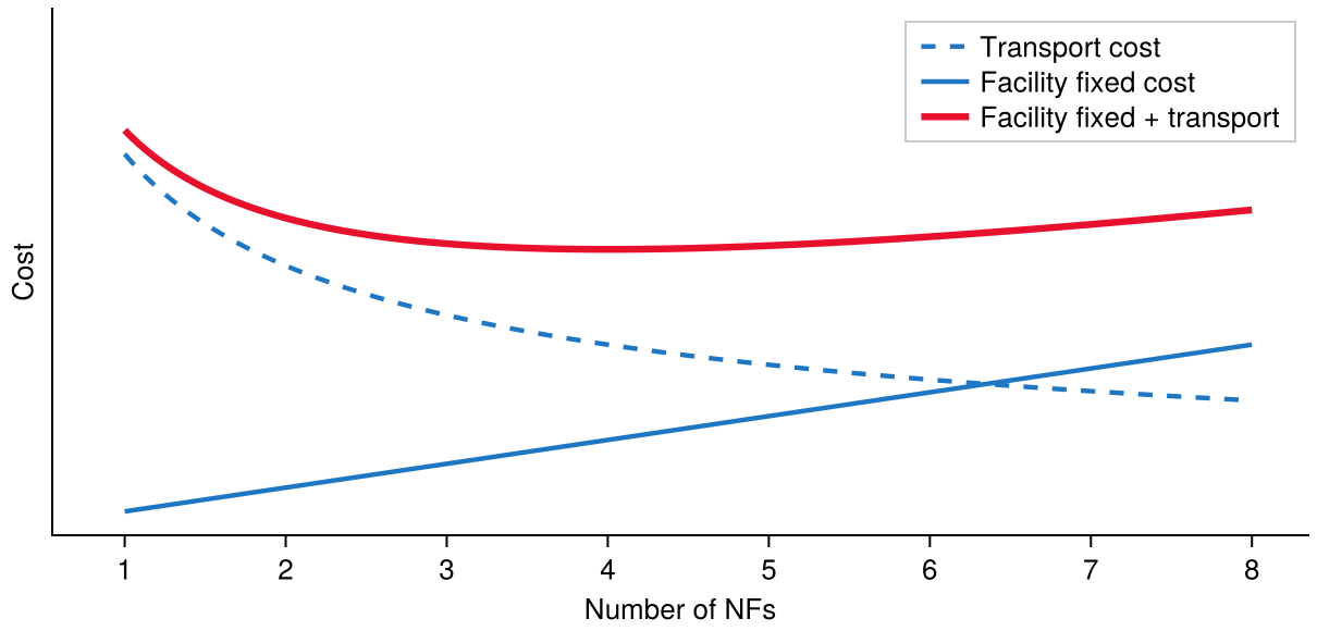
The total costs considered by the UFL are the sum of transport costs and facility fixed costs. The two costs move in opposite directions, and Fig. 1 puts them on the same axes. Transport cost falls as facilities are added, since each existing facility comes to be served by a nearer one. Facility fixed cost rises, one increment per facility. Their sum is the red curve, and it has an interior minimum: the optimal number of new facilities is where the curve reaches it.
Figure 1: Transport cost falls as new facilities are added and facility fixed cost rises, so their sum has an interior minimum. That minimum is the optimal number of new facilities.
A procedure that finds the minimum is doing two things at once, locating the facilities and determining how many of them there should be.
2. Uncapacitated facility location
NFs can only be located at a discrete set of sites. That restriction is what allows inclusion of the fixed cost of locating an NF at a site, and so the determination of the optimal number of NFs. Variable costs are usually the transport cost from the NF to and from the EFs. There is a total of 2^n - 1 potential solutions, all the nonempty subsets of sites.
minimize: total of facility fixed cost and transport cost
solve for:
(a) sites at which to locate new facilities, a subset of the n candidate sites
subject to:
(a) coverage: every existing facility is served by an open new facility
return: sites chosen and the resulting total cost
assumptions:
(a) new facilities may be located only at the given candidate sites;
(b) new facilities are uncapacitated, so every existing facility is served by whichever open site is cheapest.
Model 1: Uncapacitated facility location
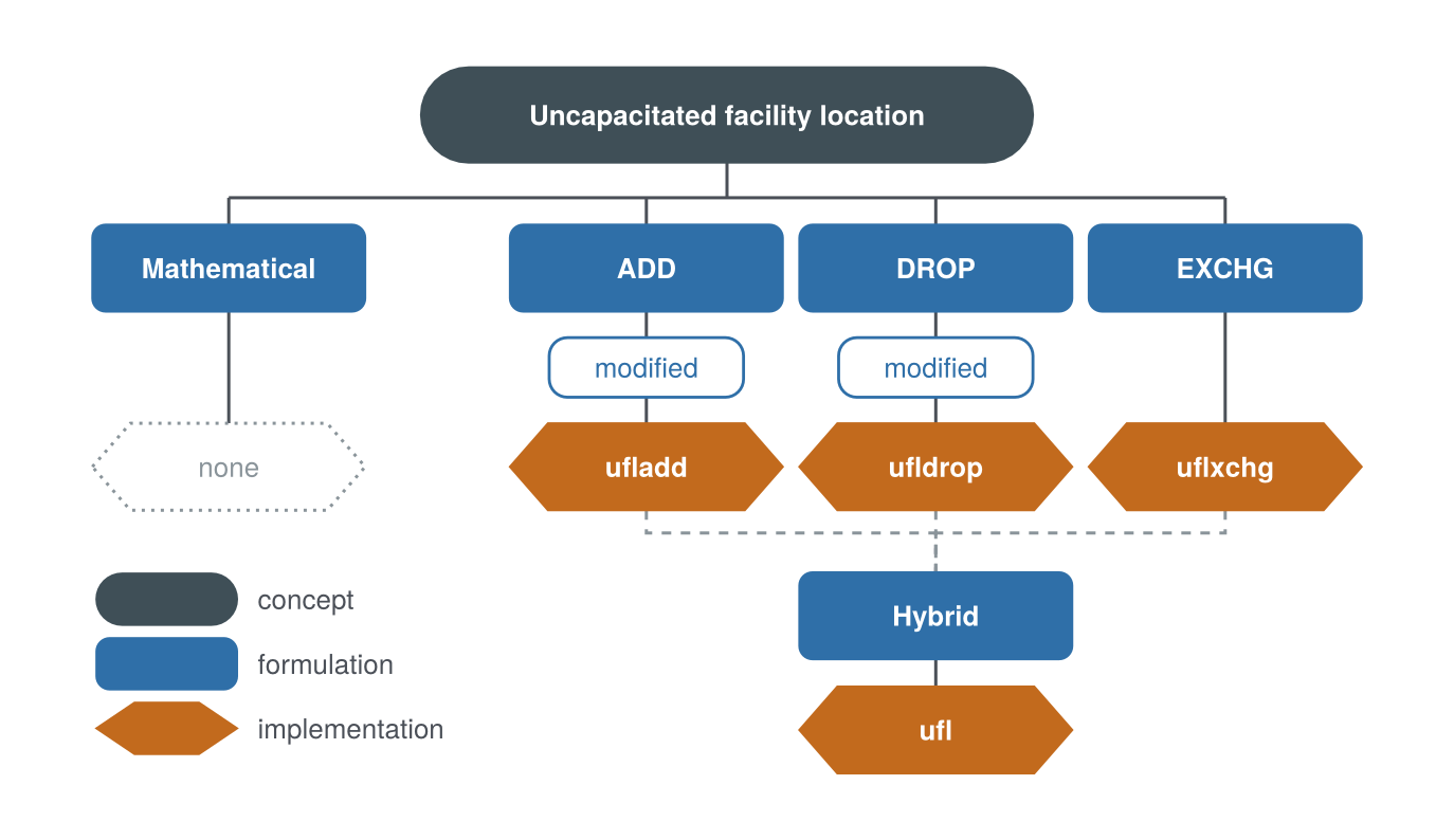
The box above is Model 1’s concept: the decision stated in words, with no symbols and no method, which is the rung every model opens in (see the Model Format Reference for more details). Additional formulation and implementation rungs of Model 1 are shown below. They never change what the concept said, but each rung commits detail the concept left open. Fig. 2 is a map of these rungs.
Figure 2: The rungs of Model 1 described in Secs. 2, 5 and 6 below. The mathematical formulation is the only one without an implementation rung. All of the other formulations are heuristic algorithms that are then implemented as Logjam functions. Modified indicates an extension of a formulation, and hybrid is a meta-heuristic built from the implementations of three other heuristics.
=set of EFs served by the NF at site i,M_i \subseteq M
c_{ij}
=variable cost to serve EF j from the NF at site i
k_i
=fixed cost of locating an NF at site i
Y
=sites at which NFs are located, Y \subseteq N
Y^\star
=minimum cost set of sites where NFs are located
|Y^\star|
=number of NFs located.
3. Construction and improvement
Most problems in logistics engineering do not admit optimal solutions, only a solution within some bound of optimal, a provable bound or optimality gap, or else the best known solution, where the search must stop when there is a need to have a solution.
A heuristic’s computational effort is split between two things:
Construction: construct a feasible solution.
Improvement: find a better feasible solution.
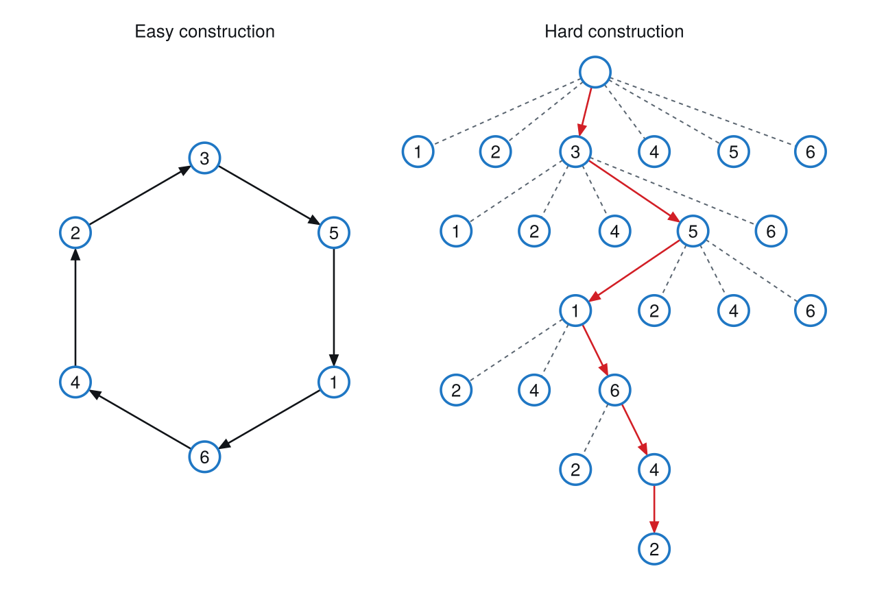
Which of the two is hard is a property of the problem rather than of the heuristic. Under easy construction, any random point or permutation is feasible and can then be improved, so the construct-then-improve cycle can be run multiple times. Under hard construction, there is almost no chance of generating a random feasible solution, because of the constraints on what a feasible solution is; randomness has to be included at the decision points as the solution is generated, in order to construct multiple different solutions, which might then be able to be improved. Fig. 3 shows one of each, built on the same six stops.
Figure 3: Two ways to construct a tour of six stops. Under easy construction any random permutation is already a tour, so one is generated and then improved. Under hard construction the tour is built one decision at a time, each step checked for feasibility, with the chosen path in red. Here both routes arrive at the same tour.
The tree is also the argument for why construction alone is not enough. Every choice eliminates everything below the branches not taken, and the choice is made on what the next step costs rather than on where it leads. That is the character of a greedy procedure: the lowest-cost next step need not belong to the lowest-cost solution. Suppose node 5 is the cheapest step from node 3 and the route through node 2 would have been far better overall. In retrospect the other choice was the right one, and there is no way of seeing that from node 3, at the moment the choice has to be made.
It is also why a purely deterministic greedy construction procedure is worth distrusting. If the next node is always whichever looks cheapest now, the procedure returns the same solution every time it runs, and running it again buys nothing. Admitting a small probability of taking one of the other branches is what makes a second run a different run.
4. Simple UFL heuristics
Being uncapacitated allows simple heuristics to be used to solve the UFL:
ADD construction: add one NF at a time.
DROP construction: drop one NF at a time.
XCHG improvement: move one NF at a time to unoccupied sites.
HYBRID algorithm: a combination of ADD and DROP construction with XCHG improvement, repeating until no change in Y. Use as the default heuristic for the UFL.
Against the division of the previous section, ADD and DROP are construction procedures, XCHG is the one improvement procedure, and the hybrid is built from both.
None of these is exact. They reach an answer that is typically within about \pm 3\% of the optimum, which is demonstrated in Lecture 2.7 by solving the same problem as a mixed-integer linear program (MILP) that returns the optimal solution. That gap is usually smaller than the error in the data going in. Demands of existing facilities are estimates, and they are nowhere near 3\% accurate. Spending effort to close the last three percent of an answer whose inputs are less reliable than that buys nothing, so from an engineering standpoint the heuristics effectively solve the problem.
The MILP is still worth having, for two reasons that are not related to accuracy. First, it gives a way to validate the UFL heuristics. Second, constraints are easy to add to a MILP and hard to add to a heuristic: holding one site open, capping a facility’s capacity, fixing the number of facilities.
The UFL can also be solved as a MILP. It is an easy MILP, whose LP relaxation is usually optimal for the strong formulation, and the MILP formulation allows constraints to easily be added, for example capacitated facility location, a fixed number of NFs, or some NF at a fixed location. Lecture 2.7 will model the UFL as a MILP, mainly to introduce MILP; the UFL hybrid algorithm is what solves most problems here.
5. ADD and DROP heuristics
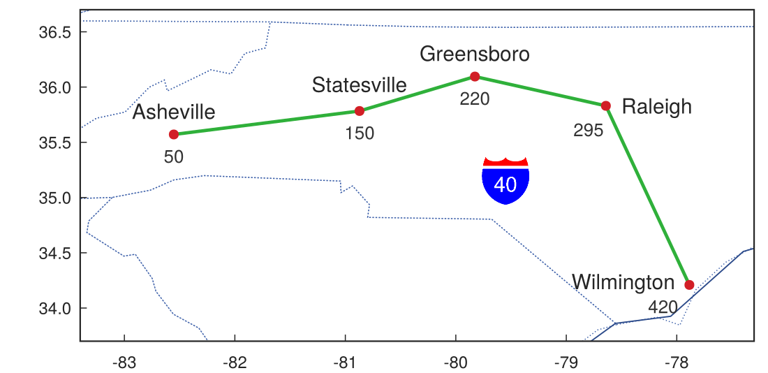
Both construction procedures can be watched on a corridor small enough to solve by hand: five cities along I-40, at the mile markers of Fig. 4. The fixed cost differs from site to site, and that is one of the advantages of the UFL. A different k_i applies at each site, where adding a fixed cost to a solution found using the ALA procedure only works when the same fixed cost applies every time a facility is added, because the new facilities can be located in a continuum of sites that cannot be individually assigned a specific fixed cost.
Figure 4: The five cities of the I-40 corridor with their mile markers: Asheville at 50, Statesville at 150, Greensboro at 220, Raleigh at 295 and Wilmington at 420.
Each pass of ADD does the same three things: try every site not yet open, keep the cheapest, and stop when none of them lowers the total. Written out, that is the ADD construction procedure.
Model 1 formulation: ADD construction
algorithm ufladd;{ input: sites N = {1,…,n} with fixed costs kᵢ, cost matrix C = (cᵢⱼ); }{ TC(Y) = Σᵢ∈Y kᵢ + Σⱼ minᵢ∈Y cᵢⱼ, total cost of the open set Y }{ output: the open set Y and its total cost TC }begin Y := ∅; TC := ∞; done := false; while done = false do begin TC′ := ∞; for each i′ ∈ N \ Y do if TC(Y ∪ {i′}) < TC′ then TC′ := TC(Y ∪ {i′}), i := i′; if TC′ < TC then TC := TC′, Y := Y ∪ {i} else done := true; end; return Y, TC;end;
Logjam exports it, and it returns the open sites, the total cost, and which cities each site serves.
Model 1 implementation: ADD construction
# Model: UFL, ADD construction# k: Fixed costs. Scalar (same cost for all) or vector (one per site).# C: n×m cost matrix where C[i,j] is cost of serving customer j from# facility i.ufladd # (k, C) -> (y, TC, W)
DROP starts from the other end. Every site has a NF, and the procedure closes whichever NF costs least to lose, until closing any of the remaining NFs would raise the total.
Model 1 formulation: DROP construction
algorithm ufldrop;{ input: sites N = {1,…,n} with fixed costs kᵢ, cost matrix C = (cᵢⱼ); }{ TC(Y) = Σᵢ∈Y kᵢ + Σⱼ minᵢ∈Y cᵢⱼ, total cost of the open set Y }{ output: the open set Y and its total cost TC }begin Y := N; TC := TC(N); done := false; while done = false and |Y| > 1 do begin TC′ := ∞; for each i′ ∈ Y do if TC(Y \ {i′}) < TC′ then TC′ := TC(Y \ {i′}), i := i′; if TC′ < TC then TC := TC′, Y := Y \ {i} else done := true; end; return Y, TC;end;
Model 1 implementation: DROP construction
# Model: UFL, DROP construction# k: Fixed costs. Scalar (same cost for all) or vector (one per site).# C: n×m cost matrix where C[i,j] is cost of serving customer j from# facility i.ufldrop # (k, C) -> (y, TC, W)
Example 1: Warehouses on the I-40 corridor
Determine where to locate warehouses along the I-40 corridor, and how many, by adding one site at a time and then by dropping one site at a time, for the five cities of Table 1.
Table 1: Mile marker and annual fixed cost of a warehouse at each of the five cities.
city
mile marker
fixed cost
Asheville
50
150
Statesville
150
200
Greensboro
220
150
Raleigh
295
150
Wilmington
420
200
Example 1(a): Adding one site at a time, by hand
Determine the sites ADD opens on the corridor, by hand, and the total cost after each pass.
Taking the transport rate and the flow as one apiece makes cost equal to distance, so the cost matrix is the distances between the cities and the arithmetic stays visible.
The procedure is worth solving by hand before any of it is written in Julia, because the table it produces is the procedure. Each pass lists every candidate set, the cost of serving each city from the nearest open site in that set, their sum c_{Yj}, the fixed cost k_Y of the sites it opens, and the total. The smallest total in a pass names the site to add, and the pass whose best total does not beat the one before it ends the procedure. The serving costs are Table 2, and the three passes are Table 3, Table 4 and Table 5.
Table 2: Cost c_{ij} of serving city j from site i.
c_{ij}
1
2
3
4
5
Asheville: 1
0
100
170
245
370
Statesville: 2
100
0
70
145
270
Greensboro: 3
170
70
0
75
200
Raleigh: 4
245
145
75
0
125
Wilmington: 5
370
270
200
125
0
Y = \{\ \}
Table 3: First pass, Y = \{\,\}: site 3 gives the smallest total.
Y
1
2
3
4
5
c_{Yj}
k_Y
c_{Yj} + k_Y
1
0
100
170
245
370
885
150
1,035
2
100
0
70
145
270
585
200
785
3
170
70
0
75
200
515
150
665
4
245
145
75
0
125
590
150
740
5
370
270
200
125
0
965
200
1,165
Y = \{3\}
Table 4: Second pass, Y = \{3\}: adding site 1 gives the smallest total.
Y
1
2
3
4
5
c_{Yj}
k_Y
c_{Yj} + k_Y
3,1
0
70
0
75
200
345
300
645
3,2
100
0
0
75
200
375
350
725
3,4
170
70
0
0
125
365
300
665
3,5
170
70
0
75
0
315
350
665
Y = \{3,1\}
Table 5: Third pass, Y = \{3,1\}: no third site beats 645, so the procedure stops.
Y
1
2
3
4
5
c_{Yj}
k_Y
c_{Yj} + k_Y
3,1,2
0
0
0
75
200
275
500
775
3,1,4
0
70
0
0
125
195
450
645
3,1,5
0
70
0
75
0
145
500
645
Y^* = \{3,1\}
# Code block 1: five cities on the corridor, and the cost of serving eachP =reshape([50, 150, 220, 295, 420], :, 1) # mile markers along I-40k = [150, 200, 150, 150, 200] # fixed cost at each siter, f =1, 1# transport rate, annual floww = r * f # monetary weightC = w *dists(P, P, 1) # cost to serve each city from each site
Site 3, Greensboro, is cheapest at 665. With it open, each city is served by whichever open site is cheaper, so adding a second site only has to beat that.
# Code block 3: the second site to add, given site 3y = [3]add =setdiff(N, y)TC2 = [sum(k[vcat(y, i)]) +sum(minimum(C[vcat(y, i), :], dims =1)) for i in add]prt(DataFrame(site = add, TC = TC2))
Site 1, Asheville, brings the total to 645. Trying a third site the same way, nothing beats it.
# Code block 4: no third site reduces the total, so stopy =vcat(y, 1)add =setdiff(N, y)TC3 = [sum(k[vcat(y, i)]) +sum(minimum(C[vcat(y, i), :], dims =1)) for i in add]prt(DataFrame(site = add, TC = TC3))
site TC
────────────
1 2 775
2 4 645
3 5 645
Sites 3 and 1, Greensboro and Asheville, at a total cost of 645.
Example 1(b): The same steps as a procedure
Determine the same answer by running ufladd, and confirm it against the hand calculation.
Running the procedure on the same data reproduces the hand calculation exactly.
# Code block 5: ADD run on the corridory, TC, _ =ufladd(k, C) # _ is the allocation, unused herey, TC
([3, 1], 645.0)
Y = \{3, 1\} at TC = 645, the same answer as by hand.
Example 1(c): Dropping one site at a time
Determine the sites DROP leaves open on the same corridor, by hand, and whether it reaches ADD’s answer.
Solved by hand on the same corridor, DROP opens every site first and then closes them one at a time.
# Code block 6: all five open, then the cheapest site to closey =collect(N)TCall =sum(k[y]) +sum(minimum(C[y, :], dims =1))drop = [sum(k[setdiff(y, i)]) +sum(minimum(C[setdiff(y, i), :], dims =1)) for i in y]prt(DataFrame(site = y, TC = drop))
# Code block 7: close site 2, then look againy =setdiff(y, 2)drop = [sum(k[setdiff(y, i)]) +sum(minimum(C[setdiff(y, i), :], dims =1)) for i in y]prt(DataFrame(site = y, TC = drop))
Sites 4 and 5 tie at 645. Taking 4 and looking once more, nothing falls below it, so the procedure stops.
# Code block 8: DROP run on the corridory, TC, _ =ufldrop(k, C) # _ is the allocation, unused herey, TC
([1, 3, 5], 645.0)
DROP ends at \{1, 3, 5\},a different solution at the same total cost of 645, and it uses three NFs where ADD used two. The difference is that site 3 no longer serves four cities: Wilmington is served by its own NF, so Asheville and Wilmington each have one and Greensboro serves the two cities between them.
Two construction procedures, run on the same data, arriving at different answers that cost the same. Neither is wrong, and neither has any way of finding the other’s solution, because each only ever moves in one direction.
ADD gives \{3, 1\} and DROP gives \{1, 3, 5\}, both at TC = 645.
6. EXCHG and HYBRID heuristics
Adding and dropping are both construction heuristics: each builds a set one decision at a time, and neither revisits a decision once taken. ADD cannot close a site it has already opened, and DROP cannot open one it has already closed.
EXCHG is the one improvement heuristic considered, and it differs from both construction heuristics by not changing the number of NFs. It takes an open site and a closed one, swaps the NF, and determines whether the swap lowered the total cost. If it did not, the solution reverts to what it was before. That is the whole of the improvement logic.
Model 1 formulation: EXCHG improvement
algorithm uflxchg;{ input: sites N, costs k and C as in ufladd, an open set Y to improve }{ output: the improved open set Y and its total cost TC }begin TC := TC(Y); done := false; while |Y| > 1 and done = false do begin TC′ := ∞; for each i′ ∈ Y do for each j′ ∈ N \ Y do if TC((Y \ {i′}) ∪ {j′}) < TC′ then TC′ := TC((Y \ {i′}) ∪ {j′}), i := i′, j := j′; if TC′ < TC then TC := TC′, Y := (Y \ {i}) ∪ {j} else done := true; end; return Y, TC;end;
Model 1 implementation: EXCHG improvement
# Model: UFL, EXCHG improvement# k: Fixed costs. Scalar (same cost for all) or vector (one per site).# C: n×m cost matrix where C[i,j] is cost of serving customer j from# facility i.# y: Initial facility set.uflxchg # (k, C, y) -> (y, TC, W)
The two loops starting at lines 9 and 10 in the above EXCHG formulation are what distinguish it from ADD and DROP: every open site is tried against every closed one, so each pass of EXCHG costs the product of the number of sites rather than the sum. In return it can reach a solution that neither construction procedure produces.
Combining the three procedures needs one change to ufladd: it has to be able to start from a set of sites that are already open, rather than always from the empty set. With that additional input argument, an improved solution can be handed back to the construction procedure and extended.
Two lines of the ADD construction formulation of Model 1 change, and nothing else does. A second argument supplies the sites already open, and a third caps how many may be opened, which is what the p-median below needs.
Model 1 formulation: Modified ADD construction
algorithm ufladd;{ two lines change; every other line is the ufladd above, unchanged }{ input gains: a set Y₀ of already-open sites, and a target count p } Y := Y₀; { was Y := ∅ } if (p = ∅ and TC′ < TC) or (p ≠ ∅ and |Y| < p) { was if TC′ < TC }
In Logjam both are keyword arguments, so a call that gives neither is the original procedure. Starting from a set of sites that are already open (termed a warm start) is what lets the procedure extend an existing network, which is the ordinary situation: facilities are rarely sited all at once, and a new one is usually added to a set already operating.
Model 1 implementation: Modified ADD construction
# Model: UFL, modified ADD construction# k: Fixed costs. Scalar (same cost for all) or vector (one per site).# C: n×m cost matrix where C[i,j] is cost of serving customer j from# facility i.# y: Initial facility set (default: empty, start from scratch).# p: Maximum facilities to select (default: nothing, no limit).ufladd # (k, C; y, p) -> (y, TC, W)
Both keywords are worth seeing used, since a warm start is the ordinary situation whenever a network already exists.
# Code block 9: warm-starting ADD, and capping the countye, TCe, _ =ufladd(k, C; y = [5]) # extend a network open at site 5yp, TCp, _ =ufladd(k, C; p =3) # or stop once three sites are open(ye, TCe), (yp, TCp)
(([5, 3, 1], 645.0), ([3, 1, 4], 645.0))
Two lines of the DROP construction formulation change in the same way. The keywords are the same two, and they mean the same things at the other end: a set of sites to start from in place of all of them, and a count to stop at.
Model 1 formulation: Modified DROP construction
algorithm ufldrop;{ two lines change; every other line is the ufldrop above, unchanged }{ input gains: a set Y₀ of sites to start from, and a target count p } Y := Y₀; { was Y := N } if (p = ∅ and TC′ < TC) or (p ≠ ∅ and |Y| > p) { was if TC′ < TC }
Warm-starting DROP is what the hybrid below does on every pass, for the reason given there, and capping the count is again what the p-median needs.
Model 1 implementation: Modified DROP construction
# Model: UFL, modified DROP construction# k: Fixed costs. Scalar (same cost for all) or vector (one per site).# C: n×m cost matrix where C[i,j] is cost of serving customer j from# facility i.# y: Initial facility set (default: all facilities).# p: Target number of facilities (default: nothing, drop until no# improvement).ufldrop # (k, C; y, p) -> (y, TC, W)
The HYBRID meta-heuristic combines all three simple heuristics. It constructs with ADD from the empty set, improves that solution by EXCHG, and then, if EXCHG changed anything, hands the improved set back to ADD and to DROP in turn. It keeps doing that until a pass leaves the solution unchanged.
Note where DROP starts. Inside the hybrid it starts from the current open set, never from the full set of candidate sites, and the reason is cost rather than quality. With about 900 three-digit ZIP codes as candidates and nine facilities to locate, dropping from 900 down to nine would take on the order of an hour even in Julia, while adding from none up to nine takes seconds. So the hybrid always constructs first and drops only from what it already holds, where the procedure can still find that a set of ten does better at nine.
Model 1 formulation: Hybrid algorithm
algorithm ufl;{ input: sites N, fixed costs k, cost matrix C }{ output: the open set Y and its total cost TC }{ construct once, then alternate improvement and construction until }{ a pass leaves the open set unchanged }begin Y′, TC′ := ufladd; Y := Y′; TC := TC′; done := false; while done = false do begin Y, TC := uflxchg with Y′; if Y ≠ Y′ then begin Y′, TC′ := ufladd with Y₀ := Y; Y″, TC″ := ufldrop with Y₀ := Y; if TC″ < TC′ then TC′ := TC″, Y′ := Y″; if TC′ ≥ TC then done := true; end else done := true; end; return Y, TC;end;
Model 1 implementation: Hybrid algorithm
# Model: UFL, hybrid algorithm# k: Fixed costs. Scalar (same cost for all) or vector (one per site).# C: n×m cost matrix where C[i,j] is cost of serving customer j from# facility i.# verbose: Print iteration costs (default: true).ufl # (k, C; verbose) -> (y, TC, W)
Example 2: Exchange and hybrid on the corridor
Determine whether exchanging a site improves on the sets that adding and dropping produced for the I-40 corridor, and what the three procedures reach when they are combined.
Example 2(a): Exchanging one site at a time, by hand
Determine whether swapping one open site for one closed site improves on either construction’s answer.
Adding gave \{3, 1\} and dropping gave \{1, 3, 5\}, both at 645. Exchange starts from one of them and tries every swap of an open site for a closed one. Starting from ADD’s pair, that is two open sites against three closed ones, so six swaps.
# Code block 10: every swap of one open site for one closed sitefTC(y) =sum(k[y]) +sum(minimum(C[y, :], dims =1))y = [3, 1]closed =setdiff(N, y)sw =DataFrame(close =repeat(y, inner =length(closed)), open =repeat(closed, outer =length(y)))sw.TC = [fTC(vcat(setdiff(y, c), o)) for (c, o) inzip(sw.close, sw.open)]prt(sw)
Closing Greensboro and opening Raleigh instead brings the total to 600. No second pass improves on it, so exchange stops there.
# Code block 11: EXCHG run on the corridor, starting from ADD's answeryadd, TCadd, _ =ufladd(k, C)yx, TCx, _ =uflxchg(k, C, yadd) # third return is the allocationyx, TCx
([4, 1], 600.0)
Y = \{1, 4\}, Asheville and Raleigh, at TC = 600.
Example 2(b): The three procedures combined
Determine what the three procedures reach run together, and which of them finds it.
Neither construction found this set. ADD opened Greensboro first because it is the cheapest single site, and having opened it never reconsidered; DROP closed Raleigh early for the same reason in reverse. Only a procedure that can move a site reaches \{1, 4\}, which is the argument for having an improvement step at all.
# Code block 12: the hybrid on the corridoryh, TCh, _ =ufl(k, C) # _ is the allocation, unused hereyh, TCh
Add: 645.0
Xchg: 600.0
Add: 600.0
Drop: 600.0
([4, 1], 600.0)
The trace shows the pattern the hybrid is built around: ADD reaches 645, exchange improves it to 600, and a further round of adding and dropping finds nothing better, so the loop ends.
Y = \{1, 4\} at TC = 600, a 7% improvement on either construction alone.
7. p-median facility location
The p-median problem is the discrete analog of the ALA procedure of the previous lecture: the same location–allocation decision, with the new facilities restricted to a discrete set of candidate sites rather than free to sit anywhere. There are no fixed costs, and the number of new facilities is fixed at p rather than determined.
It is a different model from the UFL, with its own objective and its own constraints, and its implementation is built out of the UFL heuristics. Both differences fall out of the modified ufladd: set every fixed cost to zero, and cap the count at p.
Only the construction changes. Exchange still applies unaltered, because swapping an open site for a closed one neither adds nor removes a facility, it only moves one. So the whole procedure is ADD with k = 0 and a cap, followed by exchange.
minimize: total transport cost of serving the existing facilities
solve for:
(a) sites at which to locate the new facilities, a subset of the n candidate sites
subject to:
(a) coverage: every existing facility is served by an open new facility;
(b) count: exactly p new facilities are located
return: sites chosen, and the resulting total cost
assumptions:
(a) new facilities may be located only at the given candidate sites;
(b) new facilities are uncapacitated, so every existing facility is served by whichever open site is cheapest;
(c) no fixed cost is charged for opening a site, so the count is a constraint rather than a decision.
The symbols it shares with Eq. 1 carry the meanings given there. Set beside it, the difference is the whole model: the fixed-cost term is gone, and the count that Eq. 1 determines is here a constraint.
Model 2 implementation: p-median location
# Model: p-median location# p: Number of facilities to select.# C: n×m cost matrix where C[i,j] is cost of serving customer j from# facility i.# verbose: Print iteration costs (default: true).pmedian # (p, C; verbose) -> (y, TC, W)
# Code block 20: the p-median of the corridor at p = 2p =2yp, TCp, _ =pmedian(p, C) # _ is the allocation, unused hereyp, TCp
p-median ADD: 2 facilities selected
([2, 5], 295.0)
On the I-40 corridor, asking for exactly two warehouses and charging nothing for them gives a different pair than the UFL did.
Sites 2 and 5, Statesville and Wilmington, rather than the UFL’s Asheville and Raleigh. With the fixed costs gone there is nothing to trade against distance, so the sites move outward to sit among the cities they serve.
Example 3: EMCA machine location
EMCA Industries, LLC is considering leasing machines that can be used to manufacture a single type of product. They have identified customers for the product and have estimated that they will be able to sell 12 million units per year to these customers. Each unit weighs 15 pounds and is shipped at $0.25 per ton-mile. Table 6 gives the number of customers n grouped by three-digit ZIP code across the Carolinas. They have estimated that they will be able to lease each machine for $100,000 per year; the lease cost includes the rental cost of housing it in a portion of an existing manufacturing facility. EMCA would like to know how many machines are needed to best serve their customers and where they should locate the machines, assuming that each machine can produce up to 2 million units of product per year.
Table 6: Number of customers n in each three-digit ZIP code.
zip
270
271
272
273
274
275
276
277
278
279
280
281
282
283
n
7
5
6
3
5
8
5
1
3
2
8
4
9
6
zip
284
285
286
287
290
291
292
293
294
295
296
297
298
299
n
1
2
3
3
4
3
3
2
11
5
7
2
4
2
Example 3(a): What the UFL opens, capacity ignored
Determine how many machines uncapacitated facility location opens and where, using every ZIP centroid as both a customer and a candidate site.
Five cities can be solved by hand. A real instance cannot, and it is where the heuristics earn their place. The amount of data is small enough that the arrays holding it can be created directly in Julia.
Demand is spread over the ZIPs in proportion to their customer counts, and each ZIP’s centroid stands for the customers in it. The transport rate is given, at $0.25 per ton-mile; where such a rate comes from, and how it follows from a truck’s weight and cube limits, is Transport’s subject.
# Code block 14: the cost of serving each ZIP from each candidate siterton =0.25# $/ton-mi, giveng =1.2# road circuity, lecture 2.2D = g .*dists(Pz, Pz, :mi)Cz = (fz .* rton)' .* D # $/yr to serve j from ikz =100_000.0# $/yr per machine# units/yr a machine can make; ';' keeps the echo off, and it only works# as the cell's LAST character, so the comment cannot trail the statementK =2e6;
Every ZIP is a candidate site as well as a customer, so this is a 28-site UFL.
# Code block 15: how many machines, and whereyz, TCz, Wz =ufl(kz, Cz)prt(DataFrame(ZIP = zip[yz], city =lonlat2loc(Pz[yz, :],filter(r -> r.ISCUS, usplace())).NAME, tons =round.(vec(sum(Wz .* fz', dims =2))[yz])))
Add: 1.2495292997791325e6
Xchg: 1.2482329530362058e6
Add: 1.2482329530362058e6
Drop: 1.2482329530362058e6
ZIP city tons
───────────────────────────────
274 Greensboro 18,871
294 North Charleston 13,065
282 Charlotte 18,871
296 Piedmont CDP 8,710
275 Raleigh 20,323
290 Forest Acres 10,161
The UFL opens 6 machines at a total annual cost of $1,248,233. That is the answer to the problem the UFL was given, and it is not yet the answer to the problem that was asked, because nothing in the model represents a machine’s capacity.
Example 3(b): Whether that answer is feasible
Determine whether the machines the UFL opened are within their capacity, and the smallest number of machines throughput feasibility allows.
A machine can make two million units a year, and the UFL knows nothing about that, so the first thing to do with its answer is to check it against the constraint the model never saw.
# Code block 16: what each of the six machines is asked to makeserved =vec(sum(Wz .* units', dims =2))[yz]prt(DataFrame(ZIP = zip[yz], units =round.(Int, served), pct_of_K =round.(100.* served ./ K, digits =1)))
The answer is infeasible. The busiest machine is asked for 135.5% of what a machine can make, and it is not the only one over.
How many machines does capacity require, then? Not demand divided by capacity; the throughput-feasible minimum of Eq. 4 in Lecture 1.3,
m_{\min} = \lfloor r_a\,t_e + 1 \rfloor ,
\tag{3}
where
r_a
=arrival rate
=12{,}000{,}000 units/yr
t_e
=effective processing time
=1/2{,}000{,}000 yr/unit.
The arrival rate is the rate at which work is presented to the machines, and the effective processing time is the machine-time each unit requires. The offered load is therefore r_a t_e = 6 machine-years of work per year, and
m_{\min} = \lfloor 6 + 1 \rfloor = 7 .
The floor-plus-one is doing the work. Six machines would carry an offered load of six, a utilization of exactly one, and a workstation is designed to run with its utilization strictly below one.
# Code block 17: the feasible minimum, and its p-mediante =1/ K # yr/unit, effective process timemmin =floor(Int, ud * te +1) # lecture 1.3, feasible minimumy7, TC7, W7 =pmedian(mmin, Cz)TCmin = TC7 + mmin * kz # transport plus fixed costs7 =vec(sum(W7 .* units', dims =2))[y7]prt(DataFrame(machines = mmin, total =usd(TCmin), max_pct =round(100*maximum(s7) / K, digits =1)))
So the UFL opened 6, one short of the 7 that throughput feasibility requires. Opening the seventh does not fix it: the p-median that places seven machines costs $1,249,936 a year and still asks 130.6% of one of them.
Seven is a lower bound on the count, not a feasible answer, because it counts only the total work. It says nothing about how that work is distributed, and the distribution is what a location model determines.
Example 3(c): How many machines capacity requires
Determine the number of machines at which no machine is over its capacity, and what that feasibility costs against the throughput-feasible minimum.
The obvious engineering response is to keep adding machines until no machine is over its capacity. Setting that up is a short loop, and this is where a language like Julia earns its place in the course: an experiment that would be tedious by hand is a dozen lines, and its whole history collects in a DataFrame that can be read at a glance.
# Code block 18: raise the machine count until none is over capacityres =DataFrame(machines =Int[], transport =Int[], total =Int[], max_pct =Float64[])nm, over = mmin, true# nm, not p: p is the p-median'swhile overglobal nm, over, y, TCp # a script's `while` is a soft scope y, TCp, W =pmedian(nm, Cz) s =vec(sum(W .* units', dims =2))[y] pct =100*maximum(s) / Kpush!(res, (nm, round(Int, TCp), round(Int, TCp + nm * kz),round(pct, digits =1))) over = pct >100 nm +=1end
prt(res) # Code block 19: the experiment's whole history
The sweep does not end where it might be expected to. The busiest machine stays over capacity through 10 successive counts, sitting at 111.3% for the last several of them, and only at 17 machines does every machine come within its limit.
17 machines, at a total annual cost of $1,796,918.
It took 17 machines to find a feasible solution. The throughput-feasible minimum number of machines was 7, but this number of machines would only work if each customer were able to be served from any of the machines. In this problem, each customer is allocated to only one machine, and each machine is capacity-limited. This increased the cost 44% (from $1,249,936 to $1,796,918). The reason the number of machines had to be increased so much is that the allocation did not account for capacity. In Lecture 2.7, capacity constraints will be added to the UFL model, enabling a more effective solution by accounting for machine capacity.
Example 4: Discrete retail warehouses
Determine the best nine locations for retail warehouses serving the continental United States in proportion to population, restricting them to population centroids, and compare the result with the continuous answer of the previous lecture.
The previous lecture solved this problem with ala, which may place a facility anywhere. The p-median restricts it to the three-digit ZCTA centroids themselves. That is a smaller feasible set, so it cannot do better than a perfect continuous solve; whether it does better than the continuous search is a different question, and one worth determining by running both.
# Code block 21: every US population centroid, customer and sitezr =filter!(r -> r.ISCUS ==true&& r.POP >0, uszcta3())select!(zr, :ZCTA3, :LAT, :LON, :POP)Pr =hcat(zr.LON, zr.LAT)wr = zr.POPDr =dists(Pr, Pr, :mi)Cr = wr[:]' .* Dr
# Code block 22: nine warehouses, restricted to the centroids# ';' suppresses the echo: the third return is the 882-column allocation# matrix, and printing it runs 372 characters off the page.yr, TCr =pmedian(9, Cr);
p-median ADD: 9 facilities selected
# Code block 23: naming each site by the large city nearest itcities =filter!(r -> r.ISCUS ==true&& r.POP >100_000, usplace())prt(select(lonlat2loc(Pr[yr, :], cities), :NAME, :ST, :dist))
NAME ST dist
──────────────────────────────────────────────────────────────
Lancaster CA 13.55
Athens-Clarke County unified government (balance) GA 39.78
Tacoma WA 3.60
Tyler TX 57.67
Lakeland FL 14.36
Denver CO 4.95
Rockford IL 17.19
Columbus OH 42.87
Newark NJ 2.50
The previous lecture’s continuous solve is re-run here rather than quoted, so every total is produced in the same session and they are comparable.
A random multi-start is not the only way to start ala, though, and it is not the informative one. The p-median solution is itself a feasible set of nine locations, so it can be handed to ala as a starting point; because ala descends, the run can only match or improve on it. That third solve is the one that isolates the effect of the restriction, since it is the same nine facilities freed from having to sit on a centroid.
# Code block 24: three solves of one problem, and their totalsusingRandom, Printftc(X) =sum(wr .*vec(minimum(dists(X, Pr, :mi), dims =1)))bn(x) =@sprintf("%.2f", x /1e9) # billions, always two placesRandom.seed!(4161)Xa, =ala(randX(Pr, 9), float(wr), Pr; nruns =3) # random multi-startXs, =ala(float(Pr[yr, :]), float(wr), Pr) # from the p-medianTCa, TCs =tc(Xa), tc(Xs)prt(DataFrame(start = ["restricted to centroids", "random multi-start","started at the p-median"], people_miles =bn.([TCr, TCa, TCs])))
start people_miles
───────────────────────────────────────
restricted to centroids 57.10
random multi-start 58.37
started at the p-median 56.71
Freed from the centroids, the same nine facilities reach 56.71 billion people-miles against the p-median’s 57.10, an improvement of 0.69%. The random multi-start reaches only 58.37, which is 2.22% worse than the restricted solve it is meant to beat.
The amount that the p-median is below the continuous result in the comparison actually understates the difference, because the p-median solution is restricted to a discrete set of points. Using the p-median solution as the starting point for the ALA procedure, an improvement of 0.69% was found when the solutions were allowed to move away from the discrete points, resulting in an overall improvement of 2.85% compared to the multi-start ALA solution.
This result is not always the case: it could be that the p-median solution is quite poor while one of the ALA solutions got lucky; but the result found in this example, the p-median doing better than multi-start ALA, is most common. A question then is: why use the ALA? The answer is that in most cases p-median is the better approach, and the only reason to use ALA is if there are several orders of magnitude more existing facilities than the number of new facilities, since using the p-median might be computationally difficult due to the need to store a large distance matrix. Also, the ALA is a good example of how two simple procedures, allocation and single-facility location, can be taken and, by alternating between them, effectively solve a much more complex problem; also, both the allocation and the location procedures can be easily modified, leading to a more flexible procedure than the p-median.
8. Estimating NF fixed cost
Every UFL so far has taken k_i as given. In practice, it is almost never given, and it is easy to misidentify the actual fixed costs. For example, production costs are typically split into direct and indirect costs, with indirect costs being those that cannot be directly attributed to a particular product and are instead lumped into the general category of overhead. Using overhead as the fixed cost in a UFL would not be appropriate because indirect costs typically do scale with the size of a facility, and thus would not be appropriate as a fixed cost, which by definition has to be independent of the size of a facility, essentially, the residual production costs that do not depend on the size of the facility. Instead, it is better to combine all production costs and not try to directly attribute any of them to fixed costs; fit a linear regression line and use the intercept as the fixed cost, since it does not depend on the size of the facility.
The cost being estimated is the one Eq. 1 in Lecture 2.2 put second in its ladder: production cost = procurement cost + local resource cost, where the procurement cost is the landed cost at the supplier plus inbound transport, and the local resource cost is labor and whatever is bought locally. That discussion is worth returning to, because it is what determines which costs the UFL should fold into k_i and which belong to the transport term.
Both halves fall with size. Procurement improves with scale because a larger facility buys in larger quantities, on better terms and at lower transport cost per unit; local resources improve with scale because the lumpy ones, the supervisor, the maintenance crew, the utility hookup, are spread over more output. So production cost as a whole is subject to economies of scale: it rises with the production rate, but less than proportionally.
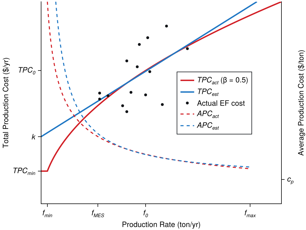
Cost from an existing facility behaves as TPC_\text{act} below: flat at TPC_\text{min} until f_\text{min} is reached, then rising as a power of the production rate. Economies of scale mean the exponent is below one, so average cost APC_\text{act} falls as the facility grows.
=scale exponent, below one under economies of scale2
k
=fixed cost
c_p
=constant unit production cost
f_\text{min}/f_\text{max}
=min/max feasible scale
f_\text{MES}
=minimum efficient scale
TPC_0/f_0
=base cost/rate.
Eq. 5 is the one the UFL needs. A straight line fitted to the same data gives TPC_\text{est} = k + c_p f, and of its two terms only k is kept. The variable part c_p f is discarded: c_p is constant, so c_p f adds the same amount per unit produced wherever the facility is put, and a term that does not vary with location cannot change which location is best. What is left, k, is the fixed cost the UFL takes, and it is combined with the variable transport cost, which does vary with location. That is what justifies the fixed-plus-transport form every UFL in this lecture has used.
Production technology has economies of scale, so total production cost is a concave function of the production rate: average cost falls as a facility gets bigger. Fig. 5 shows that curve in red, with the falling average cost dashed beneath it. A concave curve is not something the UFL can use, since the model needs one number per site. The substitute is a straight line fitted through the same data, and the number taken from it is its intercept, k, which becomes the fixed production cost.
Figure 5: Total production cost against production rate. The actual cost curve is concave, so average cost falls with scale; the fitted straight line stands in for it over the range where facilities actually operate, and its intercept k is the fixed cost the UFL uses.
The fit does not have to hold everywhere, only over the range where facilities actually operate. Nothing operates below the minimum efficient scale f_\text{MES}, because at that size the economies of scale have not been captured and the facility could not compete with larger ones, and nothing operates beyond the maximum feasible scale f_\text{max}. Between those two bounds a straight line is a good enough stand-in for the curve, and that is what justifies the substitution.
NoteWhat is the minimum efficient scale?
One reason a minimum efficient scale exists at all is lumpiness, which Lecture 1.3 Sec. 2 names as one of the three things that make production-system design hard: lumpy resources imply a minimum effective size below which it is too costly to operate. Below f_\text{MES} some of those resources are not being fully utilized, so their cost is spread over too little output and unit costs tend to be higher. At f_\text{MES} most of the lumpy resources are being reasonably well utilized, which is what the threshold marks: the production rate at which average cost stops falling appreciably.
The effect is easiest to see in the average cost rather than the total. Reading Fig. 5 toward smaller scales, APC_\text{act} starts to increase significantly for rates below f_\text{MES}, while TPC_\text{act} is merely flattening onto its floor. And the plotted data agree with the argument: every one of the actual EF production costs in Fig. 5 falls above f_\text{MES}, which is not a property of the sample but the economic claim itself. No actual plant operates below that point for any length of time, because it would not be cost effective.
Fitting that line is itself an optimization problem. Regression is a method of modeling the relationships between a dependent variable and one or more independent variables. The model is expressed as a function that “best fits” the independent variables to the dependent variable. Determining the best fit involves solving a multivariate optimization problem, where the Nelder-Mead procedure of Fig. 15 in Lecture 2.2 can be used to determine the coefficients. If the coefficients of the model are linear in the function, the method is termed linear regression. Different objective functions, termed loss functions, can be used to fit the model.
minimize: total squared deviation between the predicted and the observed response
assumptions:
(a) response is linear in the predictor over the range of the data;
(b) deviations above and below the line are equally costly, so the loss is symmetric.
Why is the L2 loss function being used? Might it be better to minimize the sum of the absolute deviations, the L1 loss\sum \bigl| \widehat{TPC} - TPC
\bigr|, instead of the square of the deviations? The two answer to different statistics of the data:
L2 loss is the only loss function that by minimizing the loss (minimum square error, MSE) allows the mean of the data to be determined; most importantly, any change in data is reflected in a change to the mean, so totals and aggregates scale correctly. Minimizing L1 loss (minimum absolute deviation, MAD) corresponds to the median of data and does not allow full information recovery, which in some cases is a good feature because it makes any estimate more robust with respect to outliers. Which of the two to fit with therefore depends on what the estimate is for: whether it will be scaled, or whether it must survive a bad data point.
What makes L2 preserve totals is a property of the fit itself: its residuals sum to zero. Because the deviations above the line exactly cancel those below, the fitted line can be subtracted from the data without disturbing any aggregate built from it, which is why L2 loss is so widely used. It is the only loss function that guarantees that balance, and so the only one that preserves totals and enables scaling. An L1 fit carries no such guarantee.
Read that way, a simple linear regression is a generalization of the average. An average is a single number chosen to best represent a set of values; a fitted line is a functional average, a best representation that is allowed to depend on a variable x. Letting it depend on more variables, or on some other form of function, changes nothing essential. The idea throughout is the same: developing a means of best representing the data.
That pairing is not new here, and it is worth recognizing where it has already been met. Model 5 in Lecture 2.1 and Model 6 in Lecture 2.1 are the same two objectives, differing by exactly one word: the equitable apartment location minimizes squared weighted distance and lands on the centroid, while the efficient one drops the square and lands on a weighted median at one of the cities. Lecture 2.1 makes the tie explicit, that “equalize-the-burden, center of gravity, arithmetic mean, and least squares are four names for the same balance condition,” and traces the same pair back to the average and median of Ex. 3 in Lecture 1.1.
The robustness this buys, and gives up, is concrete in Ex. 1 in Lecture 2.1, the minisum location along I-40. Seven North Carolina cities put the weighted median at Winston-Salem, and Asheville is the westernmost of them. Now move Asheville to California. I-40 runs there, so it is a real move and not a thought experiment, and the median location does not shift at all: the procedure never reads a mile marker, only the order of the cities and their weights, so a city that is still the westernmost carries the same weight from two thousand miles away as from the mountains. The centroid has no such protection. The same move drags it far to the west, because a squared objective is pulled by how far a point sits, not merely by which side of the line it falls on. For a location that insensitivity is often welcome; for a cost curve that must scale, it is exactly the information the estimate cannot afford to lose.
Binding Model 3 to the cost curve estimates production cost as a function of the production rate. The predictor is f and the response is the total production cost, so \alpha_1 is the intercept k of Eq. 5 and \alpha_2 is the unit production cost c_p. Taking the intercept takes the portion of production cost that does not scale with the production rate, which is exactly what the UFL charges once per facility opened; the rest, c_p f, scales with output and is the part discarded. L2 is the loss to fit with, because that k is then summed over every facility the UFL opens, and it is the mean, not the median, that keeps such a total right.
Example 5: SP3D’s fixed cost
SP3D, Inc., has been operating four hub facilities in Buffalo, NY, Pittsburgh, PA, Cleveland, OH and Detroit, MI that utilize additive manufacturing to create molds that are shipped to customers. The customers are traditional manufacturers who do not have additive manufacturing expertise in-house. Determine the fixed cost to use in a UFL for SP3D’s hubs, from the annual output and total annual production cost of each hub in Table 7.
Table 7: Annual output and production cost of each SP3D hub, exclusive of outbound transportation.
hub
molds/yr
production cost, $/yr
Buffalo
19,271
408,485
Pittsburgh
69,238
1,047,639
Cleveland
63,030
730,795
Detroit
62,117
519,401
The cost given for each hub is exclusive of outbound transportation. That exclusion is what makes the data usable. A cost figure that included outbound freight would already contain the quantity the UFL is trying to optimize, and fitting a line to it would fold transport into the fixed cost.
# Code block 25: the four hubshub = ["Buffalo", "Pittsburgh", "Cleveland", "Detroit"]f = [19271, 69238, 63030, 62117] # molds/yrtpc = [408485, 1047639, 730795, 519401] # $/yr, production only
Model 3 can now be used to fit the line, with the molds per year as the predictor and the annual production cost as the response.
# Code block 26: the fit for SP3D's four hubsk, cp =lsq(f, tpc)@show k cpfit =ŷ([k, cp], f)res = tpc .- fitdf =DataFrame(hub = hub, molds = f, actual = tpc, fitted =round.(Int, fit), residual =round.(Int, res))push!(df, ("total", sum(f), sum(tpc),round(Int, sum(fit)), round(Int, sum(res))))prt(df)
k = 198570.29338446067
cp = 8.949146412633347
hub molds actual fitted residual
─────────────────────────────────────────────────────
Buffalo 19,271 408,485 371,029 37,456
Pittsburgh 69,238 1,047,639 818,191 229,448
Cleveland 63,030 730,795 762,635 -31,840
Detroit 62,117 519,401 754,464 -235,063
total 213,656 2,706,320 2,706,320 0
k = $198,570 per hub per year. The slope, c_p = $8.95 per mold, is discarded.
The squared loss is what Model 3 is: it is in the objective, in Eq. 9, and in the model’s name. What the square is not is forced by anything around it. The line form and the numerical solve are indifferent to which loss is handed to them, so replacing the square with an absolute value changes one function and leaves the rest of the apparatus standing. That gives a different model, the least absolute deviations line, fitted to the same four hubs by the same means, and drawing both over the data shows what the choice between them costs (Fig. 6). Plotting a fitted functional form is the easiest thing a plotting library does: the coefficients are the whole description of the line, so it can be drawn anywhere the predictor runs.
# Code block 27: the same hubs under L1 loss, and both fits drawnusingCairoMakiefunctionlad(x, y) # L1: absolute, not squaredloss(α) =sum(abs.(y .-ŷ(α, x)))returnoptimize(loss, [0.0, 1.0]).minimizerendk₁, cp₁ =lad(f, tpc)@show k₁ cp₁fs = [0, maximum(f) *1.05]fig =Figure(size = (620, 380))ax =Axis(fig[1, 1], xlabel ="production rate, molds/yr", ylabel ="production cost, \$/yr")scatter!(ax, f, tpc; color =:grey25, markersize =11)lines!(ax, fs, ŷ([k, cp], fs); color =:steelblue4, label ="L2")lines!(ax, fs, ŷ([k₁, cp₁], fs); color =:firebrick, label ="L1")axislegend(ax; position =:lt)fig
k₁ = 266543.09067848907
cp₁ = 7.365570511209085
Figure 6: SP3D’s four hubs fitted twice, under L2 and L1 loss. The lines differ because squared deviation is pulled by how far a point sits from the line, while absolute deviation counts only which side of it the point falls on.
The two intercepts are not the same number: L2 puts the fixed cost at $198,570 and L1 at $266,543. Running the L1 fit through the same table as code block 26 shows which one a UFL can use.
# Code block 28: the same table under L1, where the totals disagreefit₁ =ŷ([k₁, cp₁], f)res₁ = tpc .- fit₁df₁ =DataFrame(hub = hub, molds = f, actual = tpc, fitted =round.(Int, fit₁), residual =round.(Int, res₁))push!(df₁, ("total", sum(f), sum(tpc),round(Int, sum(fit₁)), round(Int, sum(res₁))))prt(df₁)
L1 fits two of the four hubs almost exactly, which is what minimizing absolute deviation does: the line is pinned by the middle points and lets the outlying one go. But its total row no longer balances. The fitted costs fall short of the actual ones, and the residuals carry that shortfall rather than cancelling.
Put the other way round: given nothing but the molds each hub produces and the fitted line, the total production cost of all four can be recovered exactly. The individual hubs are wrong, some badly, but the aggregate is not, and that is what the fit was for. Only L2 can do it; the same recovery from the L1 line comes up $66,449 short.
That is the whole argument for L2 here, and it is not a matter of taste. The UFL charges k once for every facility it opens, so those fixed costs are added together; only a fit whose residuals sum to zero leaves such a total undisturbed, and code block 26’s total row shows the L2 fit doing exactly that. An L1 fit is the more robust of the two against a single odd hub, and it is the one that cannot be summed.
Endnotes
M. S. Daskin, Network and Discrete Location: Models, Algorithms, and Applications, New York: Wiley, 1995.↩︎
R. P. Rumelt, Note on Strategic Cost Dynamics, POL 1999-1.2, Exhibit 2, reporting a study of scale exponents across products. The general guess of b = -0.35 for manufacturing facilities is from the same page. Exhibit 2’s label column is printed one row low in the original; the bands above are aligned so that the shares sum to 100% and the general guess falls in the modal band.↩︎