3.1: Overview of Freight Transport
ISE 754: Logistics Engineering, Fall 2026
Two shipments of the same weight are not the same shipment. Their densities decide what the transport costs, and their values decide whether they go by air, road, rail or water.
1. Shippers and carriers
Few industrial engineers go to work for a freight carrier. Almost every industrial engineer working anywhere in a supply chain becomes a customer of one, and part of their job is to be the interface between the firm and the trucking, rail, or air-cargo company it hires. As a result, freight transport is taken in this lecture from the customer’s perspective rather than the operator’s: not how a carrier schedules its own equipment, but what a shipper needs to know to buy transport well.
From a terminology point of view, there is an important distinction between the terms carrier and shipper:
- Carrier: company that transports a shipment using its equipment (hired by shipper)
- Shipper: person or company that owns the shipment (customer of carrier)
This is the largest piece of terminology in freight transport, and it runs opposite to ordinary usage. Most people would call the transport company the shipper, since it is the party that ships things. In freight transport the sense is flipped: the party that operates the railcars, trucks and ships is the carrier, and the shipper is the party that contracts it. Ordering something on Amazon Prime makes the customer the shipper. A second oddity follows from the first, and it is one that students whose first language is not English have raised more than once: if the load goes by rail or by truck, why is the word shipping? Shipping in this field means any mode. It is not literally about ships.
The distinction is not merely a vocabulary lesson, because it determines which cost information the rest of Transport draws on. Almost all the costing information available is from the carrier’s point of view: what its equipment costs to operate, what it pays its drivers. The cost analysis in this course is taken from the shipper’s side instead, on the assumption that the reader is much more likely to work at a company hiring a carrier than at the carrier.
Carrier and shipper are the first of a good many terms that read oddly, and the reason they read that way is that freight transport is hundreds and in places thousands of years old. Its vocabulary goes back as far as Old English: solid, ordinary words that carry a particular meaning in this field and nowhere else, which is the opposite of how a new field sounds. Learning the terminology is part of learning the subject, and Sec. 8 collects the rest of it.
What is the most significant concept in freight transport? What a shipment is charged for transport is determined by its density. Freight capacity is a combination of the weight and the cube of a load, and in practice, most loads cube out before they weigh out. Weight is what a load physically weighs; cube is the volume it occupies. To cube out is to reach the maximum cubic volume before reaching the maximum weight capacity. The two limits arise differently. Weight capacity is set by federal law, which caps payload at 25 tons. Cube capacity is physical, but it is bounded by law as well, since a trailer may be only so wide and so tall before the load has to be flagged as oversize.
2. Transport modes and costs
As listed in Table 1, the different modes of transport can be distinguished by what it costs to move one ton, one mile. The feasibility of using each mode to transport a load is determined by whether the per-ton value of the load can bear that cost. Compared to other modes, air freight is the only one where load weight is a real cost.1 For the other modes, it is a capacity constraint, binding for dense freight but not for most general merchandise.
Water here usually means ocean transport: a container from China to the west coast of the United States. Just over two cents moves one ton one mile that way, averaged over the whole world, and since the figure varies with the origin and destination the absolute numbers are useful but not very useful. The right column is the one to keep in mind. Taking water as 1, rail is about twice as costly, and its advantage over water is that it can go where water cannot. A standard 53-foot interstate trailer costs about nine times water and about four times rail.
Everything else being equal, the ordering in the table implies a mode preference: push as much onto water as the geography allows; where there is no river and no ocean, the next best is rail; where there is no rail line, road; and last, air. What determines the outcome where there is a genuine choice is how valuable the goods are and how fast they are needed. On the ratios alone, everything that could go by rail should. What kept the traffic on trucks was dependability, or rather rail’s lack of it: a railcar loaded in Raleigh went into a black box, and until it surfaced in Los Angeles nobody knew where it was, the railroad included. Sec. 6 returns to what closed that gap.
The same ordering once drove a speculative boom. For about fifty years, canals were the Silicon Valley of their day and every government was building them, precisely because the economics of water transport are as cheap as Table 1 says. The first canals were cut in the good locations and did well; by the 1840s and 1850s they were being cut in locations that were not good. Railroads arrived at the same moment, and although rail is less efficient than a canal by the measure in the table, it is far cheaper to build, so a great many canal companies went bankrupt. Air, at 65 times water, is the other end of the same trade-off, and what sits on the far side of it is the value of the goods. A highly valued product is expensive simply to keep: it has to be financed, so every week it spends anywhere costs something in capital alone, and that cost can justify flying it. A cheap product sitting for weeks costs almost nothing, so nothing justifies the freight.
The trade-off is not always resolved the way the ratios suggest. Two weeks of national Walmart demand for a textile item, from one Southeast Asian supplier, plausibly fits on a single cargo plane, and plausibly flies, even though the items retail for $4.99 or $9.99: they are small enough that the freight is a minor share of what they sell for. Where the goods are much lower in value, getting the freight right is what matters.
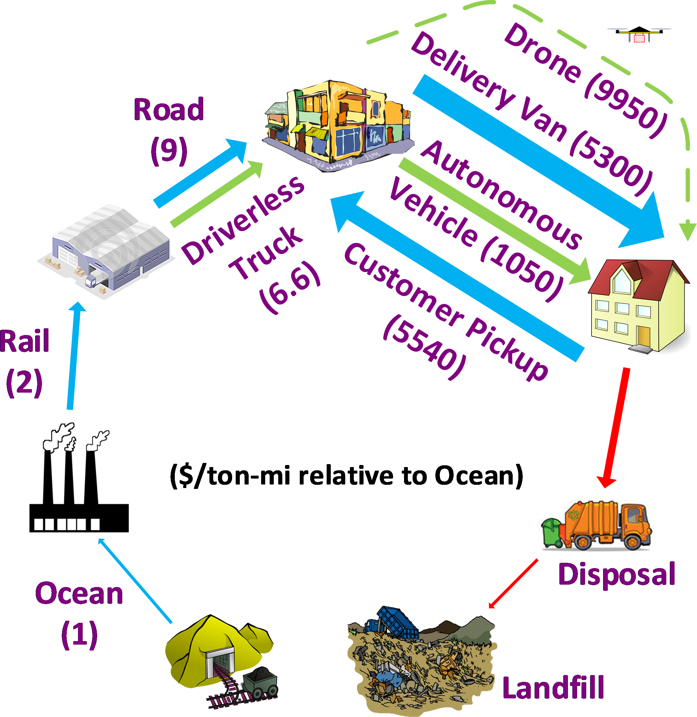
Fig. 1 takes Table 1 and expands it twice. It adds the home, which the table does not reach, and it closes the loop: goods that reach a home eventually have to be disposed of and end at a landfill. That closing leg, from the home back to the landfill, is reverse logistics, and many of the same techniques apply to it. The upstream numbers are taken from the table: ocean at 1, rail at 2, road at 9. They come from a white paper written for the material-handling industry in the fall of 2020, which needed a cost for every mode, and dirt-to-dirt logistics cost is what that exercise produced. Raw material moves by ocean where ocean is possible, then rail, then road. The interesting part of the figure is the other end: the last mile, from the distribution center to the home.
Customer pickup, at 5540, is the most expensive leg in the figure, and the reason is not the car. About 60% of that figure is the shopper’s own time, valued the way a state department of transportation values it when it evaluates an interchange: it counts the hours of driver time a project would save, at a figure in the ballpark of $12 per hour. An average store trip runs about thirty minutes, so roughly $6 of the cost is time, and the car and everything else are incidental at a dollar or two. Buying a carload of product is mostly the buyer’s personal time.
Set beside it, the delivery van is 5300, for non-perishable and non-priority goods: the kind of thing that can sit on a porch for a couple of hours, which excludes frozen food and most groceries. The two numbers very nearly match, and that is an explanation of something otherwise puzzling about 2020. When people switched from going to the store to ordering everything on Prime, nobody suddenly paid twice as much for everything, because the two legs cost about the same. The drone, at 9950, is about twice the delivery van, and the reason is worth being precise about. A drone’s operating cost is not especially high. Its payload is small, and the measure in Fig. 1 is the cost to move one ton, so a small payload is what makes the ratio large.
The autonomous vehicle, at 1050, is where the figure says the opportunity is. What makes the delivery van expensive is also what makes it inflexible: to use the driver fully, the route has to carry about 180 stops a day, which is why an Amazon delivery cannot be scheduled into a thirty-minute window and arrives sometime during the day instead. Remove the driver and put warehouses closer to houses, and the best case is about 1000, close to a five-fold improvement over having the customer go to the store. Compare that with the driverless truck, which the figure puts at 6.6 against road’s 9, a saving of a quarter or so. The two differ because of what labor is a share of. Against the cost of operating a tractor-trailer, the driver is not that much; on an Amazon delivery van the driver is almost the whole cost, so removing that driver moves the number proportionally much further. The opportunity is in the last mile, not on the interstate.
Freight transport decisions are mostly tactical, in contrast to strategic location decisions. Trucks resell readily, so a couple bought and not needed go back to a ready market, whereas a customized facility built in the wrong place may salvage for a fraction of what it cost, which makes a bad decision about where to locate, or about how many facilities to build, expensive in a way a bad decision about transport is not. What the tactical decision asks for instead is a finer resolution.
That finer resolution is what the rest of Transport is about. Location works with one monetary weight per facility, usually an aggregate over everything that facility ships. Transport works lane by lane, with different equipment on each, so the same question is asked at a much finer grain. The larger data requirement follows from the resolution rather than from the subject intrinsically requiring more data. A monetary weight is in dollars per mile and a flow is in tons per year, so the transport rate is what connects tons to dollars per mile, and its units are dollars per ton-mile. Location took that rate as given. Determining that rate is what is covered in Lecture 3.2.
In order to determine the cost to transport a shipment, a quote could just be requested from a carrier, and for one shipment that is the easiest thing to do. It says nothing, though, about whether the quote is reasonable: quoted two dollars a mile, a shipper with no reference point cannot say whether that is a good price or a bad one. In transportation everything is negotiable, which makes an independent way of arriving at what a shipment should cost an especially valuable way to evaluate the quote itself.
3. U.S. logistics costs
As shown in Table 2, the total U.S. logistics costs for 2021 were $1.847 trillion, up 11% from 2020.5 This represents 8.03% of the U.S. Gross Domestic Product (GDP). In 1981, the first full year of trucking deregulation, logistics costs were 16.2% of GDP6; in 2000, they were 10.2%,7 and in 2009 they were 7.37%, a record low percentage of GDP until 2020’s 7.22%.8 In 1981, transportation and carrying costs represented 45% and 51% of total costs, respectively9; in 2016, they represented 64% and 29% of the costs, respectively. In 2016, intercity truck transport (full and LTL) alone represents 37% of the total transportation costs and over 23% of total logistics costs, parcel has surpassed rail for the first time, and total inventory carrying costs as a percentage of the $3.202 trillion total business inventory were 15.65%.
| $ Billion | |
|---|---|
| Transportation Costs | |
| Motor Carrier: | |
| Full truckload | 332 |
| Less-than truckload | 83 |
| Private or dedicated | 415 |
| Parcel | 135 |
| Rail: | |
| Carload | 72 |
| Intermodal | 16 |
| Airfreight | 53 |
| Water | 32 |
| Pipeline | 67 |
| Total Transportation Costs | 1,206 |
| Inventory Carrying Costs ($3,20211 billion total inv.) | |
| Financial cost (WACC × total inventory) | 165 |
| Storage | 186 |
| Other (obsolescence, shrinkage, insurance, others) | 150 |
| Total Carrying Costs | 501 |
| Other Costs | |
| Carriers’ support activities | 77 |
| Shippers’ administrative costs | 63 |
| Total Logistics Costs | 1,847 |
That total is a significant share of the whole economy, and the first thing to take from the table is a proportion rather than the total itself. Freight transport is not all of logistics, but it is nearly two-thirds of what the country spends on logistics.
The rest is the cost of holding goods rather than moving them, and it divides about equally between three lines, of which the one whose name says least is the one worth explaining. Financial cost is the financing needed to cover the goods sitting in storage: inventory has to be paid for before it is sold, so it is carried the way any other asset is carried.
It can run the other way too. A grocer with thirty days to pay its supplier, selling the bananas in ten, holds what it owes for the remaining twenty days and can finance other operations with it, so the delay in payment earns rather than costs. Whether inventory is a cost or a source of funds turns on how fast it moves against how long the terms are.
Dividing the total carrying cost in Table 2 by the total business inventory it is held against gives the inventory carrying rate the data implies:
h \approx \frac{501}{3202} = 15.65\% \tag{1}
where
- h
- = inventory carrying rate.
That is the annual cost of holding inventory as a fraction of its value. The rate in Eq. 1 is what the data shows, and it is not the number to use. It is an aggregate over all logistics, dragged down by a great deal of low-value material: cement and building supplies, heavy and awkward to move and worth little per ton, so cheap to hold. That biases the average downward, and the working rule of thumb for this course is 30%. The reason is that the discrete manufactured goods considered here are typically of higher value than building supplies and the like.
That makes three design parameters worth carrying in the head: about two dollars a mile to move a truck, a circuity factor of 1.2 to turn a great-circle distance into a road distance, and a 30% inventory carrying rate. More of them accumulate over the course. What they buy is not a detailed analysis, which is always available; it is a number a level better than a guess, arrived at on one’s feet.
Table 3 puts the same total against the whole gross domestic product, year by year. The 2021 figure is about 8%, and the series holds at 8 or 9% through 2023. The record low is 2020 at 7.22%, for the obvious reason: the economy came to a standstill. The record high runs all the way back to 1981, at 16%. The parenthesized pairs are the split between transport and inventory, and they are the more interesting column. In 2021 it is about two-thirds transport and one-third inventory; in 1981 it was essentially half and half.
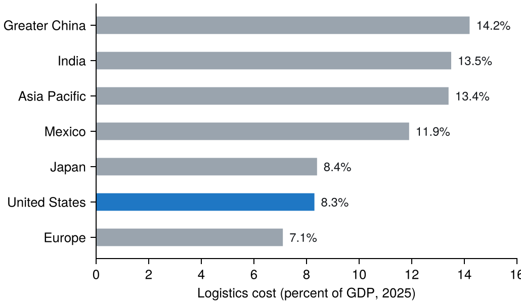
In Fig. 2, all three of the most developed economies, Europe, the United States, and Japan, have the lowest logistics cost as a percentage of GDP. What is interesting is that the United States achieves that low percentage in a different manner than Europe and Japan. The U.S. has the lowest transport cost on a per-ton-mile basis,15 but being a continental-sized country with low population density, requires about three times as many ton-miles on a per capita basis.16
Geography is the principal reason U.S. per-ton-mile transport costs are low. It has many natural harbors on both coasts, long-distance navigable inland waterways, and many 500-plus-mile hauls, which make rail feasible. The 500-mile threshold is economic rather than physical, since rail is always possible. Below it the hassle determines the choice: a truck makes a direct delivery in about a day, where rail means a day to the yard, another waiting to be loaded, a day or two moving, and a day at the far end. One day against three or four is not worth the saving. Past 500 miles the trucking cost has grown enough that it is.
Is driving on the right arbitrary? No, it has to do with logistics:
- due to the widespread use of mule trains in the U.S. for freight transport, most mule train drivers were right-handed, so they sat on the left rear mule to free their right hand to control the mules;
- prior to this, riding and driving was on the left, which freed the right hand to grip a sword;
- swords were obsolete by the time the U.S. was settled.

Start earlier. For five or six hundred years most travel was on the left, and right-handedness is the reason for that too, reaching a different conclusion. A right-handed rider carries the sword in the right hand (Fig. 3). Passing a stranger of unknown intent, keeping to the left puts the sword hand toward him and the undefended side away; passing on the right leaves that side open. Both parties protected themselves the same way, so the left was the default nearly everywhere.
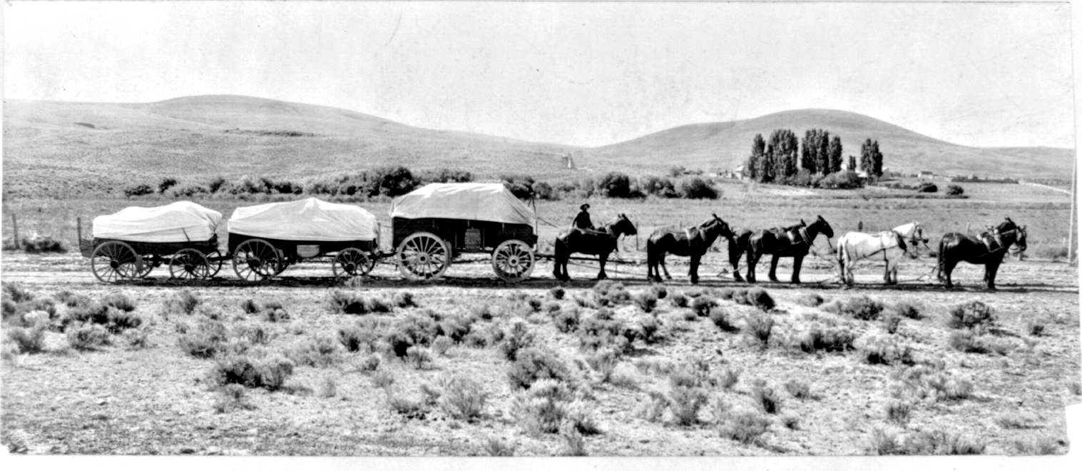
The same handedness determines the American arrangement, and how it played out is the interesting part. Until the railroads, the mule train was the main long-haul mode wherever there was no navigable river, and Fig. 4 shows the arrangement: six mules in three rows of two, and no seat. A seat would be wasted cargo space, so the driver rides one of the mules in the back row.
Which of the two he rides is determined by his hands. Sitting on the left mule of the rear pair, a right-handed driver can reach all six with the whip, and for a right-handed driver that is the efficient seat.
Guns ended the sword argument. Firearms had been in use for centuries before Europeans colonized North America, so by the time the question arose here the sword was a non-issue and the cost of moving freight was the only live consideration. Americans drove on the right. England, already on the left and locked in, did not switch, because changing the side of the road is an enormous undertaking.
Continental Europe was on the left too, until Napoleon. Taking power in France around 1800 and interested in what was new, he saw what the Americans were doing and ordered France to the right; having conquered most of the continent, he ordered the rest of it to the right as well. The map of who drives where is therefore largely a map of whom he did not conquer. England he tried and failed; Sweden he never reached; Japan is an island and was never conquered. All three stayed on the left.
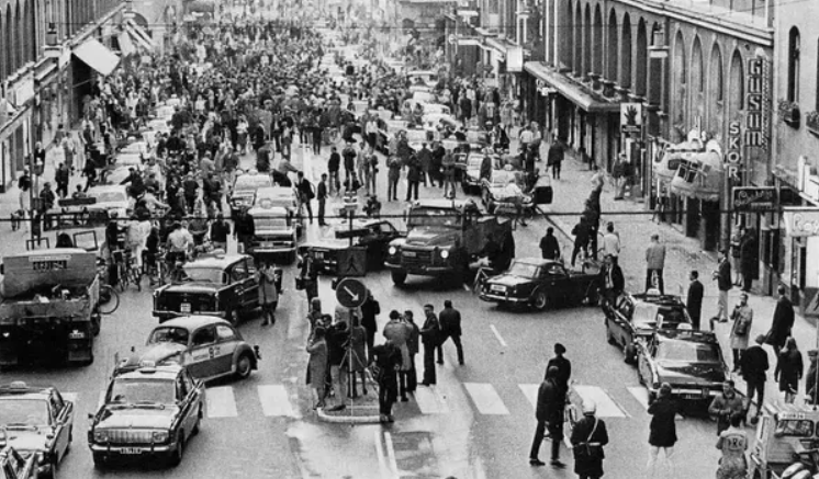
Sweden is the exception that shows the scale of it. Months of preparation went into a single Saturday midnight: every sign was ready, the country shut down for about six hours, crews were staged across it, and in those six hours the signs were changed. Fig. 5 is the Sunday morning that followed in Stockholm, a country working out how to drive. That is recent enough to be within living memory.
The point of the digression is the size of the thing it illustrates. Freight transport mattered enough to determine which side of the road half the world drives on. It was not an arbitrary flip of a coin.
4. Containerization
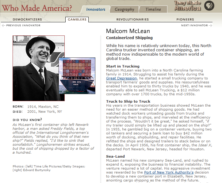
Malcom McLean is, arguably, one of the two or three people who have had the biggest impact on global trade since WWII. He patented his innovation, and then immediately gave it away. He was a trucker from Maxton, North Carolina.


Containers were the first “packetized” transport network and were developed in the 1950’s by North Carolina trucker Malcolm McLean, who started Sea-Land based in Charlotte.21 Intermodal ISO containers conform to the International Organization for Standardization (ISO) container manufacturing standards. They are used to facilitate loading and unloading at ports and to allow the container to be transported using other modes of transport like trucking and rail. The capacity of a ship is measured in TEUs (Twenty-foot Equivalent Units), an international standard.
The man in Fig. 6 is Malcom McLean. What he patented was not a box but a size of box, and, more important still, the fitting by which one box locks to another. Standardizing those two things is what let everyone else build around them. Before it, containers came in every dimension, so no port could justify specialized equipment for any of them; afterwards, cranes and ships could be designed for one shape and built to handle it efficiently. He gave the standard away rather than keeping it, and the giving away is the reason it became one.
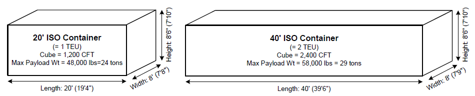
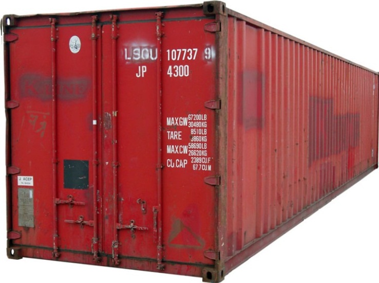
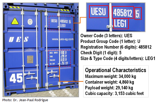
The ISO container is used to transport 90% of international trade. The standard box is 40 feet, with a cube capacity of about 2,400 cubic feet, and the half size is the 20-foot container that gives the TEU its name (Fig. 7). A 40 ft container counts as 2 TEU. One detail is worth noticing for what it says about how a standard spreads. The rest of the world is metric, and yet containers everywhere are 20 or 40 feet. This is one of the last places English units survive in international practice, and the reason is simply that the man who set the standard was American. Every box also carries its own identity, stamped on the door and read in Fig. 8.
Nothing was adopted quickly. In the late 1960s only two cases had enough value at stake to justify the new technology, and both turn on the same property: a locked container is hard to steal from. The first was the U.S. Army, shipping rifles to Europe. Freight moved in boxes was easy to lose track of and easy to pilfer; a sealed container went from the United States to its destination secure. The difficulty was the return leg, since Europe was not selling arms back. The backhaul was Scotch whisky, for the same reason and worse. Cases arriving at the port of New Jersey lost one or two to pilferage every time they were unloaded, and near Christmas the loss could run to ten or fifteen percent. A container that could be sealed in Scotland and opened at the distribution center was worth paying for. Those two cargoes carried the standard until everyone else caught up.
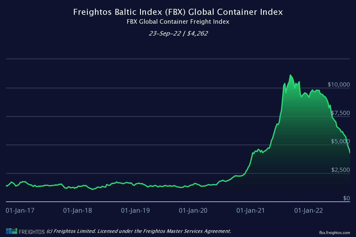
Set that against the trucking rate from Sec. 2. The $2 per mile is a stable baseline, moving little even as fuel prices do, and it wants adjusting for current cost rather than replacing. Container rates do not behave that way at all: Fig. 9 runs from about $2,000 to $10,000 and back again, which makes any analysis resting on one of them hard to trust for long. That volatility, rather than the level, is the reason ocean rates are left to the specialists and this course stays with the truck.

The fitting itself is called a twistlock, and it is as simple as it sounds. It sits in the corner casting between two stacked containers (Fig. 10); pulling the handle turns it, and the turn locks the upper box to the lower one. Unlock it and the box lifts off. That is the whole mechanism, and in some sense the twistlock is what made the global economy work: it is the piece McLean patented, and little things of that kind make a large difference to how well a system runs (a clip of a twistlock in action is worth a look26).
5. Ocean and intermodal transport
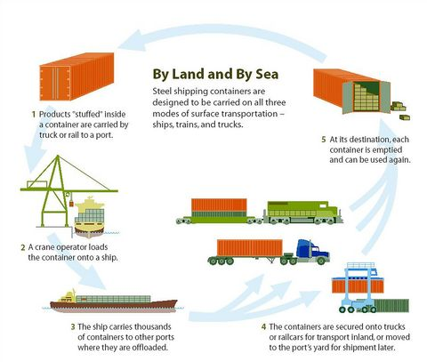
The cycle in Fig. 11 is the one a container runs. It reaches a port, specialized cranes load it onto a ship, and it is offloaded at a port at the far end. From there it goes by truck, or by rail, where two containers can be double-stacked on one flatcar, until it reaches its destination and is unloaded. Switching between more than one mode of transport this way is what intermodal means: ocean to rail to road, on the same box.
Most containers are either 20 foot or 40 foot (see Fig. 7), although high-cube 9.5-ft high and 45-, 48-, or 53-ft long containers are also available. In 2004, the cost of transporting a 40-ft container from China to the U.S. West Coast is around $2,400 (plus fees and duties) and takes 16 to 18 days, and the cost from China to the U.S. East Coast is around $4,000 (plus fees and duties) and takes 26 to 30 days. The cost of transporting a 20-ft container is 70% the cost of a 40-ft container. Containers can also be transported by rail and road. Backhaul is sometimes difficult, and the imbalance is what makes the two directions differ in cost. The number of containers traveling from the Far East to the U.S. West Coast, 11 million TEUs per year, is 2.5 times the number returning, 4.9 million TEUs.27
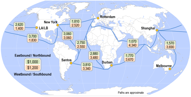
What that box costs to move is the next question, and Fig. 12 estimates it between selected ports. Shanghai to Los Angeles and Long Beach is $2,620 in the loaded direction and $1,400 coming back. That asymmetry is a complication peculiar to ocean transport: the cost one way is usually not the cost of the other, and the reason is an imbalance of supply and demand. Far more freight wants to move from Shanghai to the United States than the reverse, so the return leg is much the cheaper of the two.
How long it takes is a separate question from what it costs, and Fig. 13 answers it for the same origin. Shanghai to Norfolk is about 25 days of ocean transport. Shanghai to Long Beach is 13, and Chicago is another five on top of that, by rail. The five is the interesting number, because only a day or two of it is movement: a day or two to come off the ship and onto a railcar, two days running, and another day or two to be unloaded at the far end. Most of the time a container spends in transit, it is not in motion.
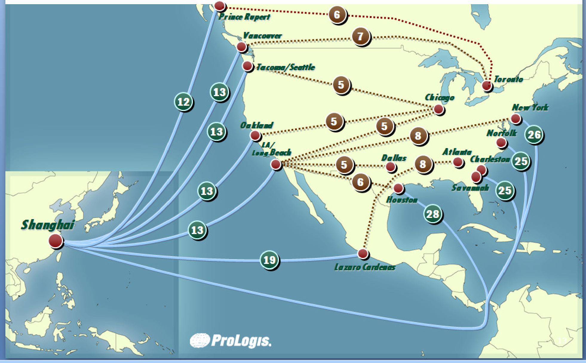
A long-haul trucker shown this figure caught that point immediately. He drove one of the routes on it and knew it did not take eight days, and he was right: the eight is from the ship’s arrival to the load being unloaded in New York, and the driving inside it is two or three days. The rest is port. A table of transit times is therefore not a table of travel times, and reading it as one overstates how far apart two places are.
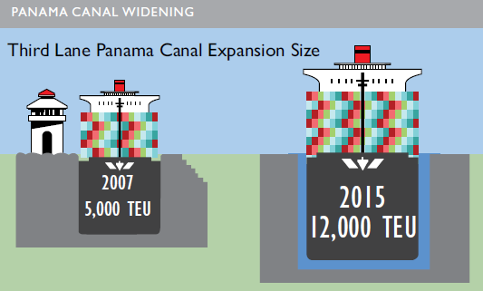
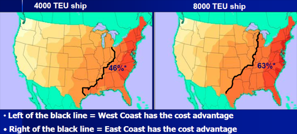
One widening of one waterway redrew where American goods enter the country. The old locks capped ships at roughly 4,000 to 5,000 TEU, the “Panamax” limit, and anything larger was “post-Panamax,” excluded outright. The new locks admit container ships of about 12,000 TEU, though some vessels remain too big regardless. A Nimitz-class carrier still cannot transit, so carriers moving between the east and west coasts of the U.S. take the long way around South America.31 Enlarging the Panama Canal let much larger ships through it, as Fig. 14 compares, and Fig. 15 shows what that did. The black line is a break-even: west of it, a load from the Far East came into Long Beach or Los Angeles and went inland by rail, and only east of it was it cheaper to run through the canal and unload at an East Coast port. Cheaper ocean capacity moved that line, and it now runs through Texas.
What the country did about it started long before the canal was finished, which is the part worth taking away. The expansion was known to be coming by the late 1990s and took ten or twelve years to build. Target, Walmart and the other large retailers began in 2000, building distribution centers and infrastructure against a change that had not happened yet, and new rail was laid from the East Coast ports to places that until then were served only from the West. Freight infrastructure has lead times measured in decades, and the response to it has them too.
It runs the other way too. Drought has since forced the canal to cut the number of ships it takes each day, and that reduction is enough that Mexico has looked at building an overland alternative across its own territory. A waterway that moved the country’s distribution map once can move it again, and the thing that constrains it need not be engineering.
6. Rail and railcar tracking
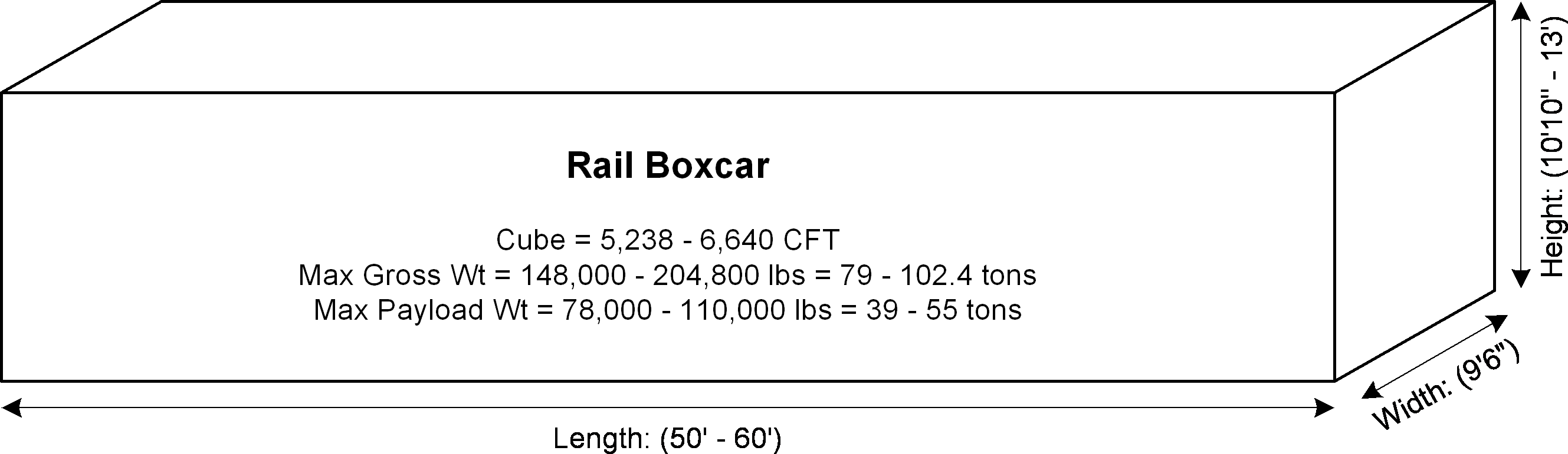
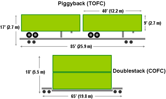
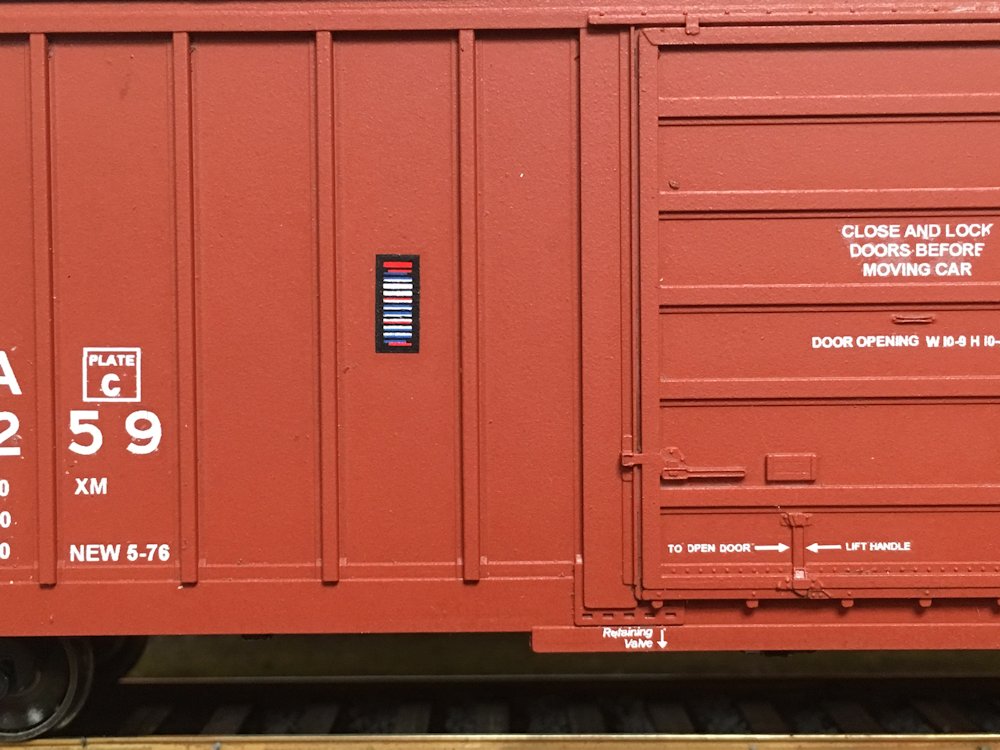
Freight can be transported by carload (CL) or less-than-carload (LCL), the rail counterpart of the truckload distinction TL (truckload) and LTL (less-than-truckload). Truck trailers can be transported on flatcars (TOFC), and ocean containers can be double-stacked on flatcars (COFC): piggyback and doublestack, the two arrangements Fig. 17 compares. Fig. 16 shows a typical boxcar. RailInc is a company located in Cary, NC that tracks the movement of railcars throughout the U.S.
Doublestacking cuts the cost of moving a container by roughly half, and Fig. 17 shows why it is not simply a matter of making the decision to do it. The complication was the bridges and the tunnels. Much of the American rail network’s grade crossing was built in the 1920s, 1930s and 1940s, when the container did not exist and no one had any reason to imagine a car standing eighteen feet tall; a rail car then was not much taller than its load.
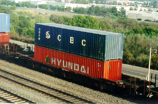
So thousands of miles of American rail carried bridges the stacked car could not pass under, and over the following twenty to forty years the railroads raised them. Not the government: private railroads, CSX among them, spending tens and perhaps hundreds of billions of dollars on work as unglamorous as lifting a bridge a few feet or lowering the track beneath it, whichever came cheaper. One such job is under way in Raleigh, a tunnel under Blue Ridge Road by the state fairgrounds, five years in so far. That is one crossing. The investment is that job repeated thousands of times.
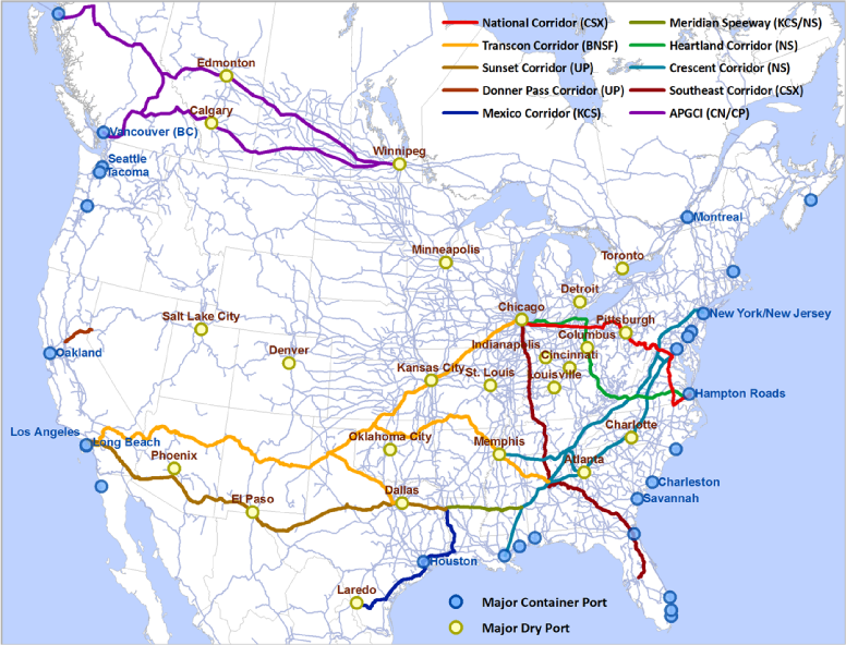
What the money bought is Fig. 18: a set of corridors on which a container can travel doublestacked from one side of the continent to the other. A box landed at Los Angeles goes on rail and stays stacked the whole way. Where it stops is notable. The eastern end of that run is Lakeland, Florida, which is the same answer given in Table 4 in Lecture 2.3 and Ex. 8 in Lecture 2.3, where Lakeland was the best location to build a warehouse in Florida; this provides confirmation of the analysis.
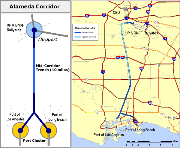
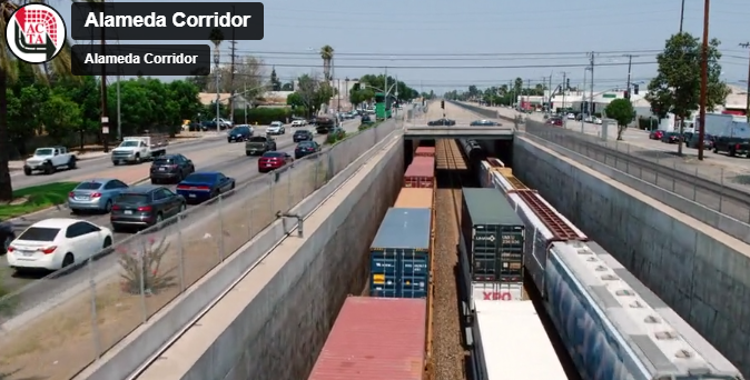
A second piece of infrastructure, finished around 2000, fixes a problem nobody had planned for. Los Angeles set its railyards about ten miles from the port. Until the Alameda Corridor was built, everything landed at the Port of Los Angeles reached those yards by truck, which meant a continuous stream of trucks through a city whose traffic was bad already. The corridor is a dedicated rail line with no grade crossings on it at all, as Fig. 19 shows: the middle ten miles run in a trench, and the surface traffic crosses over the top.
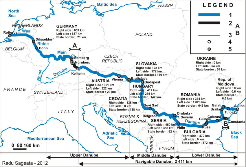
The third is older, and the scale of it is the point. The Rhine–Main–Danube axis in Fig. 20 runs from Constanța on the Black Sea to Rotterdam on the North Sea, so a barge can cross Europe on water the whole way. It was completed in 1992. Construction started in 793, on the order of the emperor Charlemagne. Freight infrastructure is not something that happens quickly.
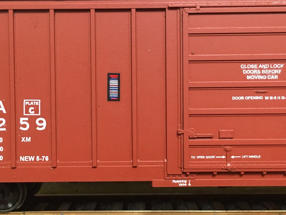
Automatic identification (Auto-ID): real-time data collection and identification. First use case that justified its development was all weather tracking of moving railcars. Kartrak was a colored bar code system developed in the mid-1960s and tested in northern Norway. The colored strips in Fig. 21 were how a railroad kept track of where its cars were. The stripes in the colored codes faded, and the technology became the first RFID (radio-frequency identification) tag, which led to the modern UPC barcode. The line from Kartrak to the supermarket is direct. The engineer who spent the winter in Norway was among the people who later developed the UPC code for the grocery industry. Automatic identification was invented to find railcars, and the checkout scanner is what it turned into.
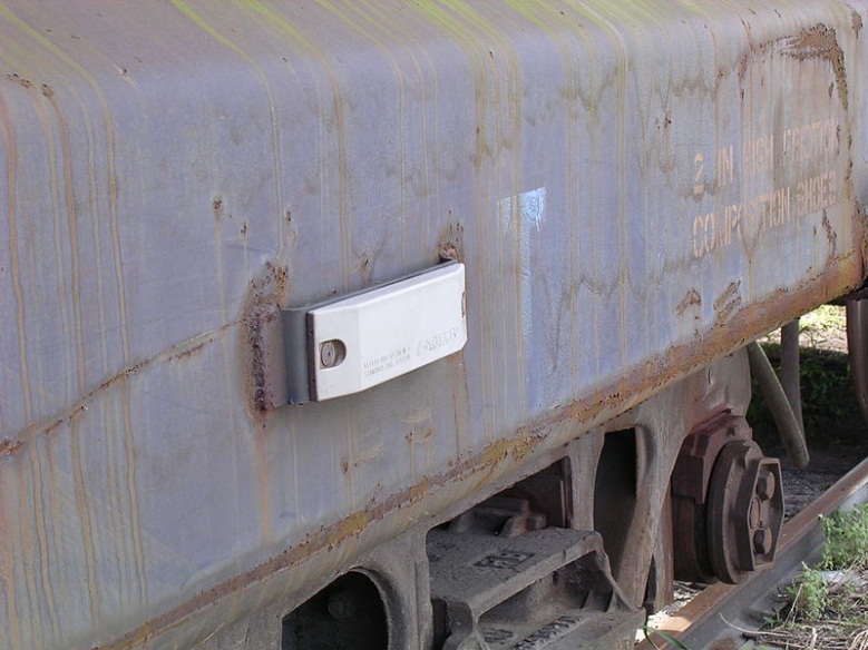
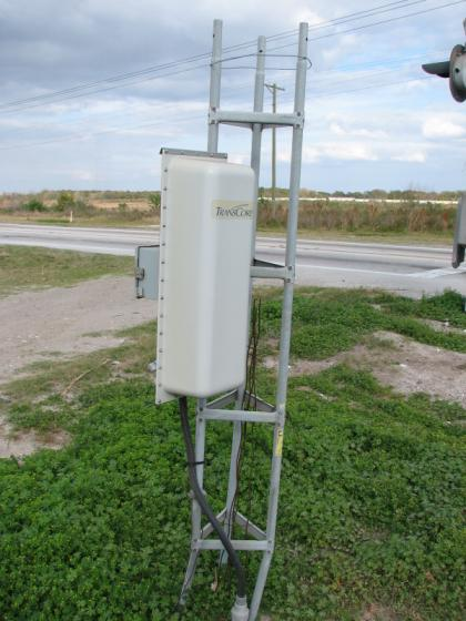
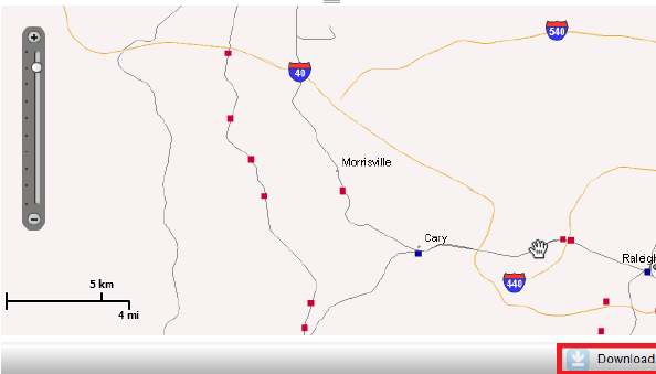
The red dots in Fig. 22 are RFID readers, and every time a railcar passes one it is recorded. A firm shipping by rail can therefore look up its own car online, see where it is at that moment, and estimate when it will reach its facility. Railinc, located in Cary, North Carolina, is a consortium supported by the railroads to run the network of RFID readers. Using Railinc, any shipper can determine the location of its shipments.
This is one of the reasons inventory costs are as low as they are, and the comparison is what makes it clear. Before about 1980, a shipper who handed a load to a railroad lost sight of it, and so did the railroad: the car was somewhere between Raleigh and Los Angeles and would arrive in one week, or two, or three. The railroad knew what happened at each yard as it happened and had no picture of the whole; the network was a black box to everyone including the people running it. Not knowing is what safety stock is for, which is Table 2’s carrying-cost line, so seeing the car is worth money long before it is worth anything else.
7. Ports and inland infrastructure
Transloading is the process of transferring a shipment from one transport vehicle to another, also known as (or similar to) transshipping. Advantages of transloading at a port prior to transport to inland distribution centers (DCs) are the following:
- the contents of four 40-ft containers fit into three 53-ft domestic containers or semi-trailers,
- the empty 40-ft containers do not need to be returned from DC, and
- probably most important, the final assignment to DCs can be delayed since the contents of the incoming container can be re-sorted based on the most up-to-date demand information, instead of shipping the full contents to a single DC.
The major disadvantage of transloading is the increased handling, both in terms of its cost and potential for damage.
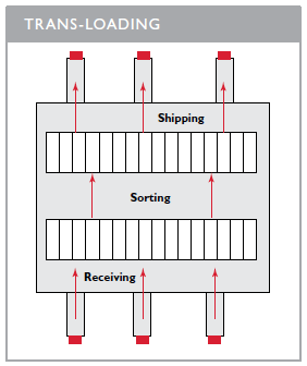
The reason the box changes size at the port is a mismatch between two standards. The 40-ft container suits the ship, and it suited the American trailer too while the legal maximum was 40 ft. From about the 1990s that maximum rose to 53 ft, and a 40-ft box on a 53-ft truck now gives up thirteen feet of length and everything it could have held.
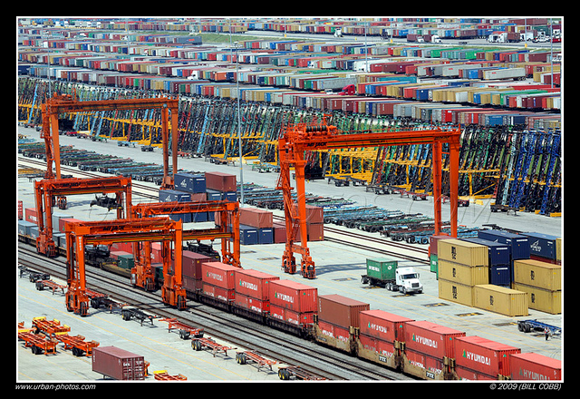
Hence a third kind of box. A domestic container never goes to sea; it moves on land only, and it is built to the size of the tractor-trailer. The large buildings beside a port are transloading facilities, and all they do is take the contents of the 40-ft boxes, sort them, and load them into 53-ft ones for the outbound leg. Fig. 23 is that building in one picture. The first saving is arithmetic: four trucks become three.
The second saving is less obvious and worth more. Sorting at the port is also a chance to determine, later, where the goods go. A box leaving Shanghai is about thirteen days from the American port and a couple of days more from the distribution center, so a firm that fixes the destination at the port is forecasting two days ahead where one that fixed it in China was forecasting three weeks ahead. A forecast made closer to the event is a better forecast, and transloading is what buys the delay.
An example makes the point concrete. Each outbound truck is going to a different distribution center, and the split is determined after the sort. A cold spell in the Northeast has raised demand for gloves there while Texas is still warm, so most of the gloves go north and fewer go to Texas. The alternative is committing to that split in China a month earlier, against a forecast nobody could make well. So transloading buys two things at the cost of one extra handling: cheaper line-haul, and the right to determine the split late.
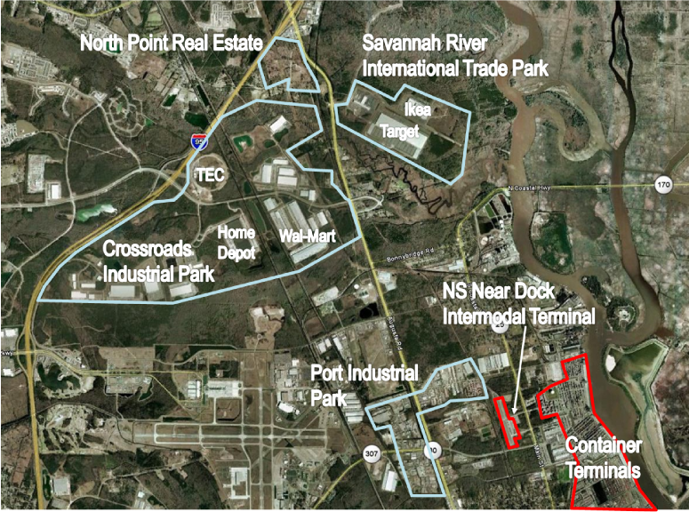
Fig. 24 is what that looks like from the air. The container terminals sit on the Savannah River, and the large buildings spread inland from them are transloading facilities: Walmart, Home Depot, Target, IKEA. This is what grows around a port that transloads, and it is not something one sees without an aerial photograph.
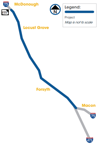
The chain that produced Fig. 25 starts at the canal. Widening it brought more freight into Savannah, that freight has to reach destinations inland and north, and the truck share of I-75’s capacity grew accordingly. The answer proposed is a road for trucks only: two barrier-separated lanes in the I-75 median, reserved for commercial vehicles, running from just south of Atlanta down toward the port. Taking the trucks out of the general-purpose lanes is expected to reduce congestion, reduce truck-and-car accidents, and cut the maintenance those lanes need. It is to open to traffic in 2032 at an estimated $2 billion.43 It is the kind of infrastructure worth having more of, and a corridor like I-95 north of Richmond is the obvious candidate.
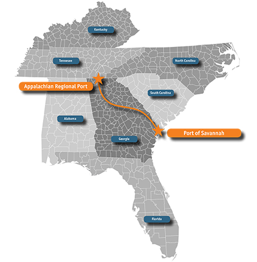
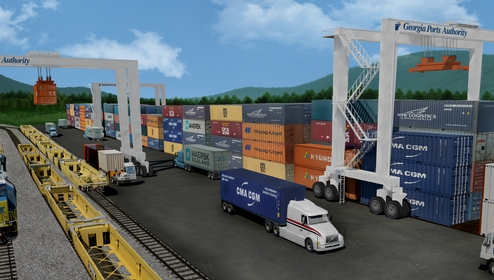
The last of these is an inland port, and Fig. 26 shows what the term means. A direct 388-mile rail route runs from Savannah to the Appalachian Regional Port in north Georgia, bypassing Atlanta’s congestion on the way, and at the far end the facility is treated exactly as an ocean port would be: boxes come off rail and onto trucks there instead of at the coast. From that point the trucks reach all of Kentucky and as far as Chicago. What it buys at the other end is less truck congestion at the port itself, and no need to transload near the coast at all. It opened in August 2018.
What everything in this section has in common is that none of it is reported anywhere a person would come across it. The raised bridges, the trench, the truck lanes and the inland port all have to be looked for. They are large, slow, expensive and almost entirely below the public’s line of sight, which is a good part of why the cost of moving a ton one mile reads like a fact of nature rather than the result of somebody’s capital program.
8. Freight terms
Freight transport uses a couple of dozen ordinary English words in particular ways. None of them is a technical term and none needs deriving; what they need is meeting once, because everything after this uses them without stopping to explain.
Demurrage: per-day fee charged by the carrier for keeping a container or trailer past the free window written into the contract
The fee exists because a trailer is cheap storage. A warehouse short of space can leave a load in the trailer it arrived in, tell the carrier it has not got round to unloading, and gain outdoor storage for nothing. So the contract sets a window, often twenty-four or forty-eight hours, and after it the carrier charges by the day, possibly hundreds of dollars a day. Nobody comes to take the trailer back; the charge is the whole of the enforcement.
Drayage: short-distance transport, typically to or from a port or rail terminal (from the dray horse that once did it)
Dunnage: material used to secure cargo inside a container (air bag, “popcorn”)
Bill of Lading: contract between carrier and shipper that serves as title for shipment
It is the paperwork the rest of the arrangement hangs on, and it is where the demurrage window and its per-day fee are written down. Much of the document is now moving onto a blockchain, on the same reasoning that moved currency there.
FOB (Free-on-Board): indicates when seller transfers title to buyer, and with it which party pays the freight
Fig. 2 in Lecture 2.2 is the four cases, seller or buyer against inbound or outbound. Lecture 2.2 works out why the choice fixes who pays for the freight without usually moving a location decision.
Reefer: refrigerated container or trailer
Common Carrier (vs Private Carrier): carrier that serves general public, as against one that carries only its owner’s goods
3PL (third-party logistics provider): firm that specializes in providing warehousing and transportation services for hire
Truck (vs. Tractor-Trailer): vehicle carrying its load on the same chassis as the cab, where a tractor-trailer is a separate power unit pulling a detachable trailer (Fig. 27)
Bobtail: tractor running with no trailer attached (Fig. 27)
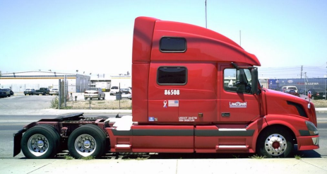
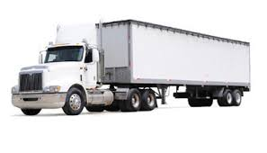
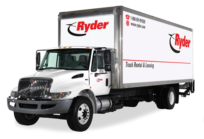
Deadheading: truck travel without a load
It is invisible from outside, because the trailer is still there whether it is full or not. The one clue from a car is acceleration: a truck pulling away from a light faster than the traffic around it is almost certainly empty. A great deal of truck travel is deadhead, and those are unproductive miles, so minimizing them is close to the objective function of running a carrier.
Doubles: one tractor pulling two trailers coupled in line (Fig. 28)
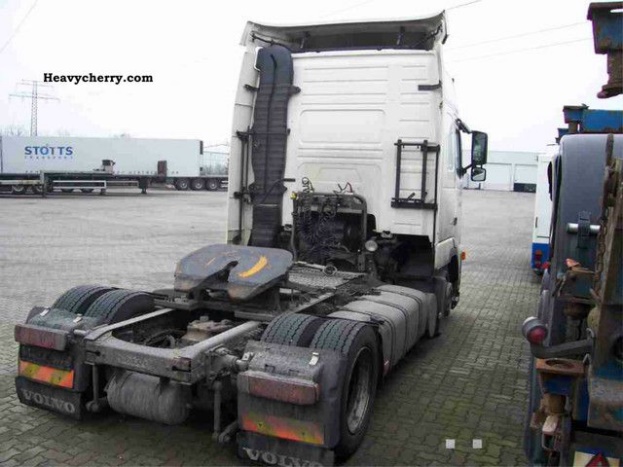
Fifth Wheel (and Kingpin): coupling plate mounted over the tractor’s rear axles, into which the kingpin under the front of a trailer drops and locks (Fig. 28)
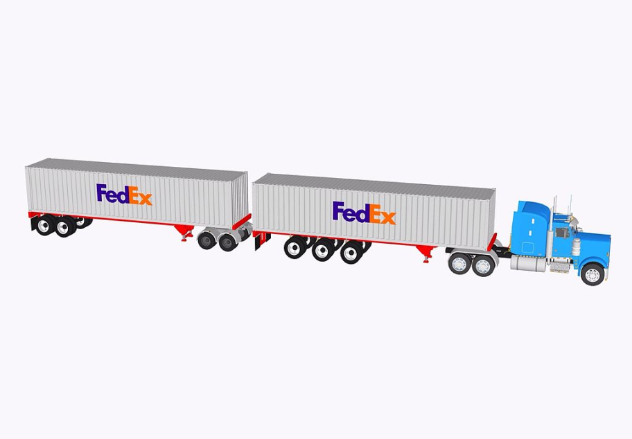
Hours-of-Service (HOS) regulations: federal limits on a driver’s time at the wheel, allowing up to 11 hours of driving within a 14-hour on-duty window, which begins after 10 or more consecutive hours off duty
Sleeper, Driver Team: allows non-stop travel with one person driving while other sleeps
This is what the hours-of-service rule leaves open: two drivers, one at the wheel and one asleep, and the truck never stops. A driver who worked such a team described running Lakeland to Los Angeles with a single refueling stop in Texas, three weeks at a time, door to door in something over thirty hours. That is faster than air cargo for the same lane, because the air route adds a drive to the airport, a wait for a plane, the flight, unloading, and the delivery at the far end. Table 1 gives the cost of a ton-mile; it does not say which mode arrives first.
Tare Weight: Tare = Gross vehicle weight – Payload
Lumper: laborer hired by a trucker to unload freight at a warehouse
The trade exists because of an assumption that turns out to be wrong. It is natural to suppose that a warehouse unloads the trucks arriving at it, with its own people. Unloading is in fact the trucker’s job, and a driver is often in no position to do it, so an outsourced trade of casual labor has grown up around the dock, hired by the trucker rather than by the warehouse. It is the kind of thing that is invisible from a manager’s office and obvious at the dock.
Endnotes
The air industry encodes this threshold explicitly. IATA’s volumetric divisor fixes the density at which a shipment stops being billed on the space it occupies and starts being billed on what it weighs; see Maersk, Air Cargo Chargeable Weight, 10 March 2025, https://www.maersk.com/logistics-explained/transportation-and-freight/2025/03/10/air-cargo-chargeable-weight, and DHL Global Forwarding, Calculating Chargeable Weights, https://www.dhl.com/us-en/home/global-forwarding/freight-forwarding-education-center/calculating-chargeable-weights.html. Lecture 3.2 gives the figure and sets it beside the trailer and the container.↩︎
M. G. Kay, Challenges and Opportunities Associated with Using Autonomous Vehicles and Drones for Home Delivery, 2020, unpublished. Some of the numbers here are revised from the ones in the report; the analysis behind them is unchanged.↩︎
The air figure is not from the 2020 report, whose dirt-to-dirt framework does not extend to air cargo. It is the 2018 average freight revenue per ton-mile for domestic scheduled air carrier service, from U.S. Department of Transportation, Bureau of Transportation Statistics, National Transportation Statistics, “Table 3-21: Average Freight Revenue Per Ton-mile,” accessed 21 September 2026; the same source and year give 4.23 cents for Class I rail. Cargo revenue there covers scheduled and charter property revenue and mail revenue, and excludes carriers that did not report both financial data and a full year of traffic data, so the figure is a U.S. domestic average set against an international ocean rate. The relative column is that cost divided by the cost of water.↩︎
M. G. Kay, Challenges and Opportunities Associated with Using Autonomous Vehicles and Drones for Home Delivery, 2020, unpublished. As with Table 1, some of the numbers in the figure are revised from the ones in the report; the analysis behind them is unchanged.↩︎
John Schulz, “State of Logistics 2022: Out of sync,” Logistics Management, 2022 https://www.logisticsmgmt.com/article/state_of_logistics_out_of_sync.↩︎
Schulz, J.D., “State of Logistics 2010: Business logistics costs fall 18.2 percent,” Modern Material Handling, Jun. 9, 2010.↩︎
Trunick, P.A., 2005, “Can we hold the line on logistics costs?” Logistics TODAY, Penton Media.↩︎
John Schulz, “State of Logistics 2022: Out of sync,” Logistics Management, 2022 https://www.logisticsmgmt.com/article/state_of_logistics_out_of_sync.↩︎
Logistics Costs and U.S. Gross Domestic Product, Federal Highway Administration, U.S. Dept. of Transportation, Aug. 25, 2005, http://ops.fhwa.dot.gov/Freight/freight_analysis/econ_methods/lcdp_rep/index.htm.↩︎
CSCMP’s 33rd Annual State of Logistics Report, as reported in John Schulz, “State of Logistics 2022: Out of sync,” Logistics Management, 2022 https://www.logisticsmgmt.com/article/state_of_logistics_out_of_sync.↩︎
Private inventories: Annual average, seasonally adjusted, Federal Reserve Bank of St. Louis, Series ID A371RC1Q027SBEA. https://fred.stlouisfed.org/series/A371RC1Q027SBEA#0 (accessed 2022.09.26).↩︎
Record low.↩︎
2024 from CSCMP’s 36th Annual State of Logistics Report (released 3 June 2025), which put U.S. business logistics costs at $2.58 trillion; 2025 from the 37th (June 2026), which put them at $2.40 trillion and gave the split as 61.8% transportation, 30.4% inventory carrying and 7.8% other. Each row records the year as first published. CSCMP revises the whole series with each report, so the current basis differs: the 37th restates 2022 at 10.2%, 2023 at 8.4% and 2024 at 8.3%, against the 9.04%, 8.76% and 8.8% shown here. The difference is a change of basis, not an error in either figure.↩︎
Global Logistics Costs and Third-Party Logistics Revenues for Key Regions and Countries, Armstrong & Associates, Inc., with International Monetary Fund GDP data; 2025 figures, updated 20 April 2026, accessed 18 September 2026. The basis is not Table 3’s: A&A put U.S. logistics costs at $2,545 billion for 2025 where CSCMP’s 37th report gives $2.40 trillion, which is 8.3% against 7.8% of GDP for the same year. The chart is built to compare across countries, which is what this section uses it for, and is not comparable with the tally above.↩︎
Rail is the mode whose rates can be compared across countries on one basis. CPCS, International Comparison of Railway Freight Rates, prepared for the Railway Association of Canada, 31 January 2023, Fig. 4, gives 2021 freight revenue per revenue ton-mile in purchasing-power-adjusted U.S. cents: United States 4.66, against Spain 7.26, Italy 8.12, France 8.13, Germany 9.73 and Japan 12.19. Of the ten countries surveyed, three are lower still: Canada at 4.16, China at 3.51 and Russia at 3.26.↩︎
F. M. B. A. Furtado, “U.S. and European Freight Railways: The Differences That Matter,” Journal of the Transportation Research Forum 52(2), Summer 2013, pp. 65–84. Its 2009 figures put U.S. road and rail together at 2.90 trillion ton-miles, which is 4.24 trillion tonne-km, against 2.05 trillion tonne-km for the EU27. Per head that is 13,817 tonne-km against 4,109, a factor of 3.4.↩︎
http://fineartamerica.com/featured/knight-riding-horse-sword-cartoon-aloysius-patrimonio.html.↩︎
Freight team, ca. 1905. Library of Congress, Prints and Photographs Division, https://www.loc.gov/item/2013647269/. No known restrictions on publication.↩︎
https://www.quora.com/What-are-some-rare-photos-of-world-history/answer/Ryan-Bales-5.↩︎
PBS, They Made America, http://www.pbs.org/wgbh/theymadeamerica/whomade/mclean_hi.html.↩︎
Taggart, S., 1999, “The 20-Ton Packet,” Wired, Oct.↩︎
Container photograph, Wikimedia Commons, http://en.wikipedia.org/wiki/File:Container_01_KMJ.jpg; identification system, Jean-Paul Rodrigue, The Geography of Transport Systems, http://people.hofstra.edu/geotrans/eng/ch3en/conc3en/container_identification_system.html.↩︎
Freightos Baltic Index (FBX), https://fbx.freightos.com/freight-index/FBX.↩︎
The first two readings are his own. The third is the FBX global index as reported on 7 September 2026 by IndexBox, Weekly Container Shipping Rates, which quotes the index’s latest weekly update at $3,520; it is a trade report quoting the index rather than a reading taken from the index directly, the index’s own chart being available only behind a sign-up.↩︎
Wikipedia, Twistlock, http://en.wikipedia.org/wiki/Twistlock.↩︎
Twistlocks explained, mdiddams, https://www.youtube.com/watch?v=wXXnEzXAip4. Linked rather than embedded: this project renders every lecture with
embed-resources: true, which inlines an iframe’s source as a scriptless snapshot, so an embedded player shows a black frame and does nothing.↩︎Economist, 2004, “Boxed in and clogged up,” Economist, Oct. 14.↩︎
Cycle diagram, Smithsonian, America on the Move, http://americanhistory.si.edu/onthemove/collection/image_826.html; CenterPoint aerial, http://www.flickr.com/photos/49394874@N08/5125215424/.↩︎
Jean-Paul Rodrigue, The Geography of Transport Systems, after Drewry Shipping Consultants. Rates are for full container loads and include the base ocean shipping rate, port charges at both origin and destination, fuel surcharges and all other surcharges. The site moved from
people.hofstra.edu/geotrans; the figures are those of 2010.↩︎Gregory Arnold, Global Supply Chain Trends and the Impact on North American Distribution Markets, Prologis, presented to the U.S. Department of Transportation Federal Highway Administration, 15 July 2009.↩︎
The 2016 locks are 1,400 ft long by 180 ft wide, but Nimitz- and Ford-class carriers are blocked by the width of their sponsons; see Center for Maritime Strategy, “Can the Greatest Maritime Infrastructure Project Ever Provide Even More Benefits to the United States?” (February 2025). In March 2026, USS Nimitz transferred from Bremerton to Norfolk via a 12,400-nautical-mile route around South America rather than through the canal.↩︎
The 2015 Expansion of the Panama Canal and the Impacts on the North American Container Fleet, John Vickerman, 2013. The third set of locks opened on 26 June 2016, after the presentation the figure comes from was given, which is why it is drawn as a forthcoming change.↩︎
NAIOP Research Foundation, The New Age of Trade: The Americas. The foundation’s copy at
naiop.org/foundation/newageoftrade.pdfno longer resolves, checked 18 September 2026.↩︎Jean-Paul Rodrigue, The Geography of Transport Systems: Piggyback (TOFC) and Doublestack (COFC) Train Cars, https://transportgeography.org/contents/chapter5/intermodal-transportation-containerization/container-tofc-cofc/, and 40-Foot Containers Doublestacked on a Rail Car, https://transportgeography.org/contents/chapter5/rail-transportation-pipelines/doublestack-railcar/. The site moved from
people.hofstra.edu/geotrans, and these are the current locations of the same two figures, checked 18 September 2026.↩︎Jean-Paul Rodrigue, The Geography of Transport Systems, Major North American Rail Corridors Improved since 2000, https://transportgeography.org/contents/chapter5/rail-transportation-pipelines/rail-corridors-north-america-improvement/. The site moved from
people.hofstra.edu/geotrans, and this is the current location of the same map, checked 18 September 2026.↩︎Alameda Corridor Transportation Authority, https://www.acta.org/about/who-we-are/.↩︎
Radu Săgeată, Rhine–Main–Danube transcontinental axis, 2012, as credited on the map itself; reproduced at https://www.researchgate.net/figure/Rhine-Main-Danube-transcontinental-axis-1-Navigable-rivers-2-Navigable-canals-A_fig1_278023765. See also Rhine–Main–Danube Canal, Wikipedia, https://en.wikipedia.org/wiki/Rhine%E2%80%93Main%E2%80%93Danube_Canal. The map’s numbered legend is not expanded on the figure; what the passage uses is the continuous navigable line from Rotterdam to the Black Sea.↩︎
Image and history: http://vanderheide.ca/blog/wp-content/uploads/2017/09/063.jpg and Ernie Smith, The Railroad Barcode That Came Before the UPC, Tedium, 5 September 2017, https://tedium.co/2017/09/05/kartrak-railroad-barcode-history/.↩︎
Tag and reader photographs, Wikimedia Commons, http://en.wikipedia.org/wiki/File:AEItag.jpg and http://en.wikipedia.org/wiki/File:AEIreader.jpg; reader map from Railinc’s IRFi user guide, https://www.railinc.com/irfidoc/help/IRFiUserGuide.pdf.↩︎
NAIOP Research Foundation, The New Age of Trade: The Americas. The foundation’s copy at
naiop.org/foundation/newageoftrade.pdfno longer resolves, checked 18 September 2026.↩︎Jean-Paul Rodrigue, The Port of Savannah Logistics Cluster, https://transportgeography.org/?page_id=8490. The site moved from
people.hofstra.edu/geotrans, and this is the current location of the same study, checked 18 September 2026.↩︎Georgia Department of Transportation, I-75 Commercial Vehicle Lanes, project fact sheet, https://www.dot.ga.gov/systems/ProjectDocuments/0014203/I-75%20CV%20Lanes%20Fact%20Sheet.pdf. The address previously published for this document no longer resolves; this is the department’s current fact sheet for the same project.↩︎
Status checked 18 September 2026. The project is in design and environmental review, with construction expected to begin in 2027 and finish about 2032, at roughly $2 billion for 41 miles of barrier-separated lanes through Henry, Spalding, Butts, Lamar and Monroe counties. The slide’s 2029 opening and $1.8 billion estimate were current when it was made.↩︎
Georgia Ports Authority, Appalachian Regional Port, https://gaports.com/facilities/inland-ports/appalachian-regional-port/, accessed 18 September 2026. CSX’s New Georgia Inland Terminal Planned news release, and its Appalachian Region Port map and terminal image at
industrialdevelopment.csx.com, no longer resolve, checked 18 September 2026.↩︎The straight truck from Ryder’s reservation vehicle images,
reservations.ryder.com, and the tractor-trailer from Manheim’s vehicle images,manheim.com.au.↩︎Doubles, Wikimedia Commons, https://commons.wikimedia.org/wiki/File:40_foot_container_turnpike_double.jpg; fifth wheel, heavycherry.com.↩︎