2.1: Types of Location Problems
ISE 754: Logistics Engineering, Fall 2026
“We fail more often because we solve the wrong problem than because we get the wrong solution to the right problem.” — Russell Ackoff1
Facility location is a good place to begin the study of logistics engineering, not only because determining the location a facility has far-reaching and long-term implications for the effective operation of a logistics network (e.g., the “Why are cities located where they are?” callout, below), but because it is physical and visual in a way that inventory and most other topics are not. A location problem cannot be solved until its objective has been determined, and since a location problem can be drawn on a map, the trade-offs between competing objectives can be seen directly. That makes it an unusually clear vehicle for illustrating the modeling ideas that recur throughout the course: what an objective is, how a single objective can hide a choice, and how what at first glance seem like incompatible concerns can be combined so that one objective can be optimized.
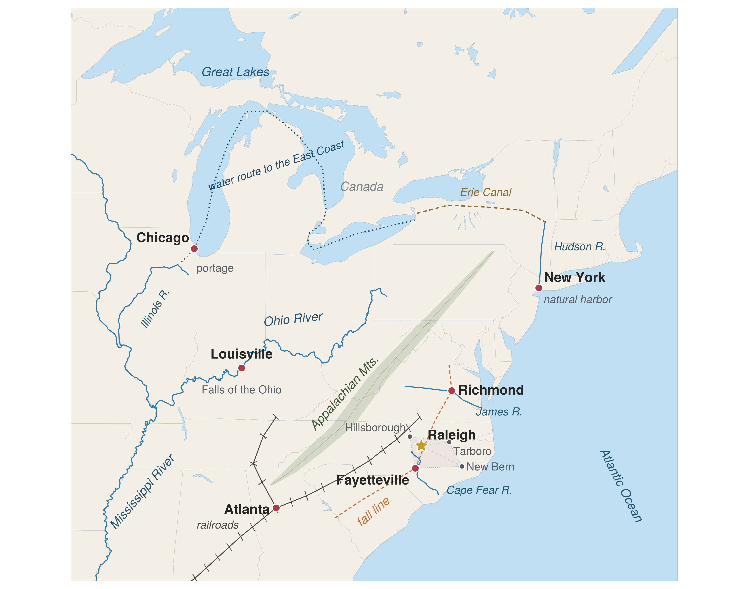
Why are cities located where they are? For many cities, logistics is a principal reason. As can be seen in Fig. 1, Atlanta grew because it was the first place where a railroad could get around the southern end of the Appalachians, opening a gateway to the west. New York has a near-perfect natural harbor, and the later construction of the Erie Canal provided water access all the way to the Great Lakes. Many cities’ location has to do with transshipment: the need to move cargo from one mode of transport to another. Chicago sits at the short portage between the Great Lakes and the river network that reaches the Mississippi, so cargo arriving by ship had to be unloaded and reloaded there. Many cities, including Richmond and Fayetteville, sit at the falls of a river, the farthest point upstream that boats could reach before goods had to be offloaded and carried overland. Louisville is located at the only falls on what is otherwise all-water travel between the headwaters of the Ohio and the Gulf of Mexico. The recurring pattern is a break in transport where goods must be handled, which is exactly where the labor and then the city accumulate. Raleigh is an exception whose logic is still locational: it was placed near the center of the four principal North Carolina towns at the time.3 Each of these towns was competing to be the capital, so that no delegation had to travel too far to the capital.
Two problems are used in this lecture to illustrate different modeling ideas. The first, locating hot-dog stands on a beach, separates competitive from cooperative location decisions, and shows why minimizing customer travel is not, by itself, an adequate objective. The second, a couple choosing where to live between two cities, introduces the trade-off between equity and efficiency. The idea to carry through both, and through the course, is that choosing the objective, not solving it, is what makes a logistics problem interesting; the couple sharpens that to a single result, that cooperation is what lets the linear objective be the right one. Solutions for both problems are developed as a series of models, each written in the callout form introduced in Lecture 1.1, so that what changes from one model to the next is visible at a glance.
1. Taxonomy of location problems
The single most important idea in facility location is a modeling distinction, not a location result: for most private-industry applications, minimizing the sum of total distances is the most appropriate objective, and it happens to be linear; being linear it is reasonable to assume that transport cost increases in direct proportion to distance, because, for example, a truck driver is paid roughly by the mile; also, such linear minisum problems can be much easier to solve compared to other location problems. In many public or personal applications, cost increases faster than distance, so the objective is nonlinear. For example, most people would prefer twenty thirty-minute driving trips to one ten-hour trip, even though the total distance is the same; whether that nonlinearity is modeled or ignored changes what a model of the situation actually represents.
A taxonomy of the different types of location problems is shown in Fig. 2. Cooperative location decisions are used to minimize the total system costs of multiple facilities owned by a single firm instead of just minimizing the cost of each of the firm’s individual facilities. These decisions are possible when the impact of the location of other firms’ facilities does not significantly impact the location of one’s own facilities. Cooperative location problems that optimize something other than this linear minisum (minimizing the maximum cost, for instance) are grouped as “nonlinear.” Competitive location decisions arise when the value of locating an individual facility is impacted by the location of facilities owned by other firms. In what follows, only transport-oriented minisum location problems are considered because these problems are the ones that most benefit from a simple analysis using transport-cost minimization as the sole criterion, and the assumption that costs are directly proportional to distance is usually reasonable; local-input-oriented location problems arise when transport costs are not the dominant cost associated with the location decision, and are typically solved using different techniques.
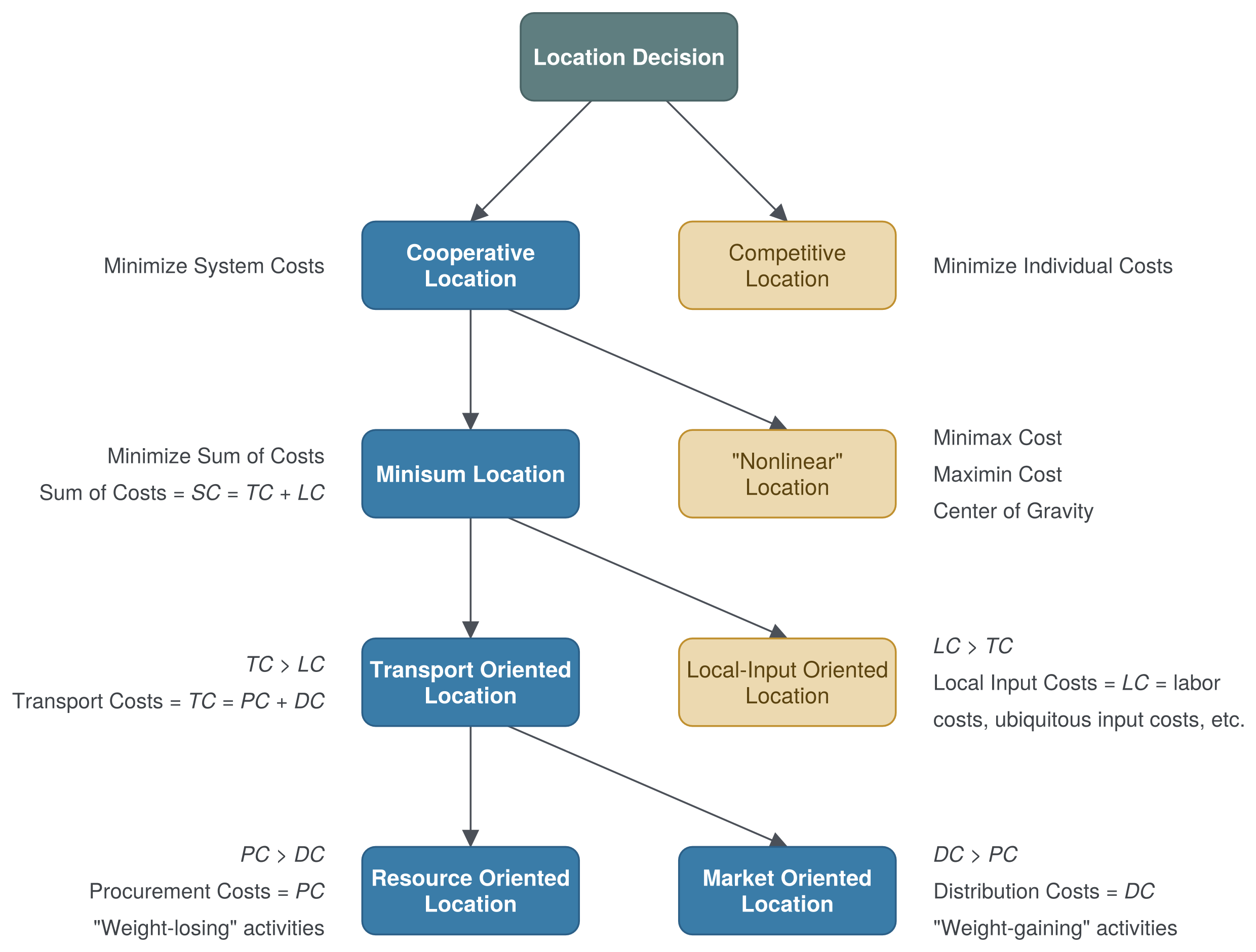
A transport-oriented location problem is termed resource-oriented when the cost of procuring a good exceeds the cost of distributing it. Consider the production of metal from ore: the mining facility must be close to the source of the raw material, because once the metal is extracted from the surrounding rock it is much cheaper to transport. The problem is termed market-oriented when the cost of distributing a good exceeds the cost of procuring it. Consider an Amazon distribution center, where large tractor-trailers bring the goods in, but many small delivery vans deliver them to customers.4
The next two sections present two problems that follow from the use of this taxonomy: the first (see Section 2) compares competitive with cooperative location, and the second (see Section 3) concerns comparing a “nonlinear” objective with a minisum objective for a cooperative location problem. Together, they make the case that choosing the objective, rather than the geometry, is what makes a location problem interesting. The mechanics of actually solving the minisum problem are taken up in Section 4, and the other types of location problems named in the taxonomy are illustrated in Section 5.
2. Competitive vs cooperative location
Competitive location. Consider a beach a mile long. Customers are spread uniformly along it, which is a reasonable approximation because beachgoers tend to set up not next to each other but as far apart as they can, so they end up roughly evenly distributed. A single hot-dog stand somewhere on the beach captures the entire market, since it is the only one. Suppose a second stand opens, selling an identical product at the same price. Assuming each customer walks to the nearer stand, where should the second stand locate, and where do the two end up?
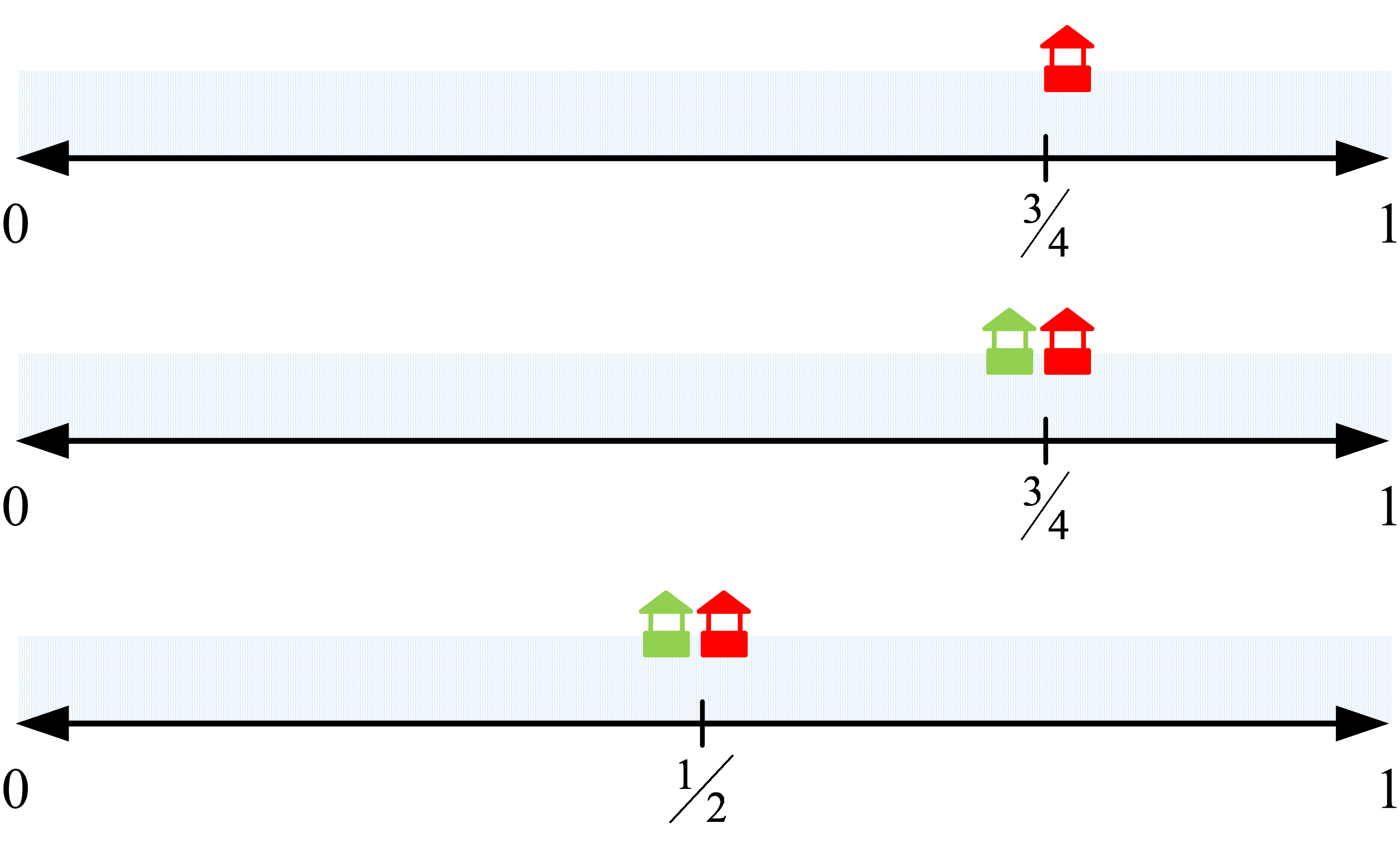
A second stand placed just to the busier side of the first captures the larger share of the market. But the first stand, being a mobile cart, can then move to reclaim that share, and the second responds in kind. Because each stand is free to relocate and each wants the larger share, the only stable outcome is both stands side by side at the center of the beach (Fig. 3). This is the competitive result, an instance of Hotelling’s law,5 the tendency of competitors to cluster together rather than spread out: fast-food outlets at the same interchange are the everyday version of it. The competitive problem is stated in Model 1.
Harold Hotelling, the economist behind this eponymous law, left Columbia for the University of North Carolina at Chapel Hill in 1946, where he founded its Department of Mathematical Statistics6 (Gertrude Cox founded NC State’s Department of Experimental Statistics in 1941, one of the country’s oldest7).
maximize: share of the market a stand captures
solve for:
(a) where each stand locates, any point along the beach.
subject to: none
return: pair of stand locations
assumptions:
(a) two stands are owned independently, so each competes for customers;
(b) customers are spread uniformly along the beach;
(c) both stands sell an identical product at the same price;
(d) each customer buys from the nearer stand.
Cooperative location. On the competitive beach, each stand maximizing its own share of the market drives the two together and both stands sit at the center of the beach. These are the worst possible locations with respect to how far customers have to walk. Now suppose on a different beach, the competition is removed. A single resort buys the beach and grants a single owner the exclusive right to sell hot dogs on it. Freed from the fight over market share, the owner would want to place two stands at locations that minimize customer travel so that excessive walking discourages the least amount of customer demand (Model 2). Changing who owns the stands changes the objective; the remaining assumptions of uniform demand, an identical product, and nearest-stand choice carry over unchanged.
maximize: share of the market a stand captures minimize: average distance a customer travels to reach a stand
solve for:
(a) where each stand locates, any point along the beach.
subject to: none
return: pair of stand locations
assumptions:
(a) the two stands are owned independently, so each competes for customers a single owner controls both stands;
(b) customers are spread uniformly along the beach;
(c) both stands sell an identical product at the same price;
(d) each customer buys from the nearer stand.

The optimal placement is now the quarter and three-quarter marks (Fig. 4): customers in the first half of the beach use the first stand, those in the second half use the second. Cooperation is unambiguously better for customer travel.
How far customers walk. Each model returns a pair of stand locations, not a walking distance; how far the average customer actually walks is a separate quantity, worth computing on its own. Doing so measures how much cooperation shortens the walk, and the computation shows exactly what the uniformity assumption buys.
On the competitive beach both stands sit at the center, so a customer at position x walks |x - X/2| each way, a one-way distance that ranges from 0, for a customer at the middle, to X/2, for one at either end. Assumption (b) of Model 1, customers spread uniformly, makes the average of that range its midpoint, X/4, so the average round trip is \bar d_{\text{comp}} = 2 \cdot \frac{X}{4} = \frac{X}{2} .
On the cooperative beach the stands sit at the quarter marks, and assumption (d) of Model 2 sends each customer to the nearer stand, so each stand serves its own half of the beach from that half’s center. Within a half of length X/2 the one-way walk again runs uniformly, by assumption (b), from 0 to X/4, averaging X/8, so the average round trip is \bar d_{\text{coop}} = 2 \cdot \frac{X}{8} = \frac{X}{4} , half the competitive figure. Uniformity is doing the work in both derivations: drop it and each distance would have to be weighted by how many customers stand there, and the clean midpoint, hence the clean halving, would not survive.
Customer’s choice. Shorter walks are not the whole story, though. With competition gone, nothing stops the single owner from raising the price of the hot dogs. The gain in shorter walks is paid back at the counter, so minimizing travel alone is no longer an adequate objective: it ignores the very thing that the loss of competition changes.
The objectives so far belonged to the sellers. To see what the customer faces, put the two beaches side by side: the competitive beach, with its stands at the center and a price held down by competition, and the cooperative beach, with its stands at the quarter marks and the higher price a single owner can charge. A customer choosing between them weighs a cheaper hot dog against a longer walk, and the two are measured in different units. Comparing them requires making dollars and miles commensurate: a per-mile cost c that evaluates how much a customer values a mile of walking saved.
minimize: customer’s total cost of a hot dog: the price paid plus the round-trip walk valued at c dollars per mile
solve for:
(a) which beach the customer visits, the competitive or the cooperative.
subject to: none
return: beach chosen
assumptions:
(a) two beaches operate side by side: on the competitive beach both stands sit at the center and competition holds the price down; on the cooperative beach the stands sit at the quarter marks and the single owner charges more;
(b) customers are spread uniformly along each beach;
(c) each customer values a mile of walking at their own rate c;
(d) on either beach, a customer buys from the nearer stand;
(e) customer picks a beach before picking a spot on it.
For the first time the decision-maker in Model 3 is not a firm but a customer, and the model changes with the decider: the return line names a choice of beach, not a pair of stand locations. The optimal decision rule follows from writing out each beach’s average total cost and comparing them, with each ingredient traced to a named element of the model. Assumption (a) fixes the two offers: let the competitive beach charge p_1 and the cooperative beach charge p_2 > p_1. By assumption (e), a customer picks a beach before picking a spot on it, so the walk that enters the comparison is the average round trip; assumption (b), customers uniform along each beach, together with the nearer-stand rule of assumption (d), is exactly what lets the averages derived earlier stand in for that walk, X/2 with both stands at the center and X/4 with stands at the quarter marks. Assumption (c) supplies the personal rate c that converts walking to dollars. Each beach’s average total cost is then its price plus its walk valued at c per mile, C_{\text{comp}} = p_1 + c\,\frac{X}{2}, \qquad C_{\text{coop}} = p_2 + c\,\frac{X}{4} . The cooperative beach is the better choice when C_{\text{coop}} < C_{\text{comp}}, and the rule falls out of the algebra: p_2 + c\,\frac{X}{4} \;<\; p_1 + c\,\frac{X}{2} \;\;\Longleftrightarrow\;\; \underbrace{p_2 - p_1}_{\text{premium paid}} \;<\; \underbrace{c\,\frac{X}{4}}_{\text{walking saved}} \;\;\Longleftrightarrow\;\; c \;>\; \frac{4\,(p_2 - p_1)}{X} . The middle form is the rule in words: choose the cooperative beach exactly when the walking it saves, a quarter-beach round trip valued at c per mile, is worth more than the price premium it charges. Customers who value money more than walking, with small c, take the cheap stands at the center; customers who value convenience, with large c, pay the higher price for the shorter walk. Neither beach is better outright, and both can fill: the threshold c = 4(p_2 - p_1)/X splits the market, and each customer’s own rate determines which side of it they are on.
The modeling idea to carry forward is the weight itself, the per-mile cost c. Combining evaluate and distance in a single objective forces the two to be made commensurate, and there is no way around choosing the weight that does it. Optimizing distance first and evaluate second (sequential optimization) is not valid, because the best beach on one criterion is not the best on the other. A multi-objective formulation is possible, but its output is a set of trade-off solutions, and choosing among them still requires a weighting.
3. “Nonlinear” vs minisum objectives
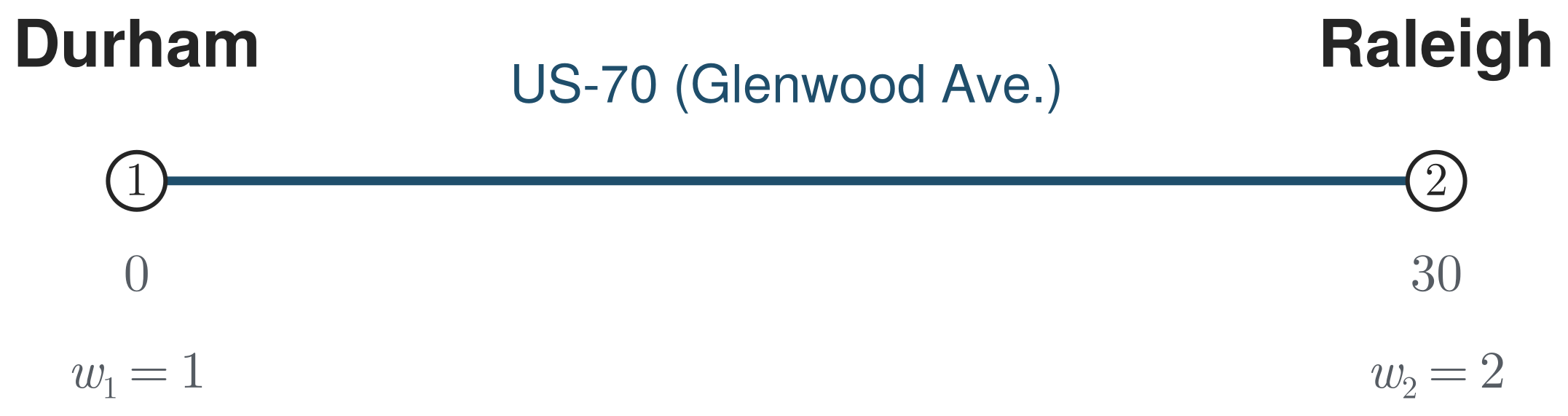
In this section, two types of modeling objectives are examined in relation to their impact on a couple’s location decision when looking for an apartment after moving to the Triangle area in North Carolina. The couple is hypothetical; the choice they face is not. The couple is choosing an apartment somewhere along the roughly thirty-mile US-70 corridor between Durham and Raleigh. One partner makes a single trip a day to work in Durham; the other both works and attends school in Raleigh, making two trips a day. Taking the number of daily trips as the weight of each destination, Durham has weight 1 and Raleigh has weight 2. Placing Durham at mile 0 and Raleigh at mile 30, at what location x (in miles along US-70) should they look for an apartment? One location turns out to be fair and another cheap, and they are not the same place. Fig. 5 is worth a moment for how little it contains: the whole decision is a single number on a line, and the two objectives that follow disagree only about which number.
Start with fairness. Where can the couple live so that neither partner is stuck driving more than the other? Equalizing the two partners’ weighted travel means w_1\,x = w_2\,(30 - x), \qquad 1\cdot x = 2\,(30 - x) \;\Rightarrow\; x = 20, the point two-thirds of the way from Durham to Raleigh. For two points this fair location is x = w_2 a_2/(w_1 + w_2), the weighted mean.
solve for:
(a) location x of the apartment, any point along the corridor.
subject to:
(a) equity: the two partners’ weighted travel is equal, so neither is stuck driving more than the other.
return: location x of the apartment along the corridor
assumptions:
(a) apartment can be located anywhere along the corridor;
(b) Durham trip has weight 1 and the Raleigh trips have weight 2.
The callout has no objective slot at all, which is what makes it a feasibility model: it states a fairness condition the location must satisfy, not a quantity to make small. Turning that condition into an optimization answers a question typically unasked: why is squared distance the quantity so many methods minimize? Written out, equalizing the burdens is the balance condition \sum_i w_i(x - a_i) = 0, \tag{1}
the weighted pull to the left set equal to the weighted pull to the right. Nothing has been optimized here either; this is just the fairness requirement stated directly, which is the natural way to write it down.
An equation of this “set the net pull to zero” form is a first-order condition. The name comes from calculus: at the bottom of a valley the ground is level, so the slope of whatever is being minimized is zero there, and setting a slope to zero is a condition on the first derivative.
A word of warning before going further, because what comes next runs against the grain of the approach used through the rest of the course. The normal practice, in this course and in engineering generally, is to start from an objective, write down the quantity to be made small, and differentiate it to reach a condition like this one. That is exactly the order followed, again and again. Here the opposite is done, and only this once: the balance condition happened to come first, because equalizing the burdens was the intuitive thing to write down directly, so the logic can be run backward, asking the question in reverse: Eq. 1 is the zero-slope condition of what function? Recovering an objective from a condition is a useful trick for seeing where squared distance comes from, but it is a detour, not the method used here. Once the answer is in hand, the reasoning returns to objective-first for good. Recovering a function from its slope is integration, and the function whose derivative is \sum_i w_i (x - a_i) is \min_x \; \sum_i w_i (x - a_i)^2 , \tag{2}
up to a constant factor that does not move the minimum. So the balance point is exactly the minimizer of total weighted squared distance. The square is not a modeling choice made for convenience or smoothness; it is simply what the balance condition integrates to, and differentiating it returns Eq. 1. Solving gives the weighted centroid, or center of gravity,
x^* = \frac{\sum_i w_i a_i}{\sum_i w_i} , \tag{3}
which for the couple is x^* = 20. The physical reading is a seesaw: because squared distance has a slope proportional to distance, the level balance point is where the weighted distances offset, exactly the center of mass.
This same fact sits under the ordinary average, and the connection is worth making explicit. The plain mean of a set of numbers is their balance point, the value at which the deviations sum to zero, and squared error is precisely the objective whose first-order condition that balance is. That is why least-squares regression minimizes the sum of squared errors rather than something else: the square is the antiderivative of “make the deviations balance.” The average introduced in Lecture 1.1 (Ex. 3 in Lecture 1.1) is this centroid with equal weights, the equitable solution, and the median introduced alongside it is the efficiency solution. Equalize-the-burden, center of gravity, arithmetic mean, and least squares are four names for the same balance condition, and integrating that condition is what puts the square in all of them.
Changing the fairness condition into a quantity to minimize is a genuine change of objective, not merely a rewording, so it defines a new model: a refinement of Model 4 that solves the same problem in a form a standard optimizer can accept. Refining a model this way, from stating the condition a solution must satisfy to naming an objective to optimize, is a routine and powerful move, and here it also exposes the tie to least squares.
minimize: total weighted squared distance from the apartment to the two workplaces
solve for:
(a) location x of the apartment, any point along the corridor.
subject to: none, the equity condition having been replaced by the objective above
return: location x of the apartment along the corridor
assumptions:
(a) apartment can be located anywhere along the corridor;
(b) Durham trip has weight 1 and the Raleigh trips have weight 2.
The fair location fixes how the driving is shared, but not how much driving there is in total. A couple that cares more about the total mileage, rather than about who bears the driving burden, would pose the question the other way around: they might instead minimize the total distance driven, adding the mileage up rather than balancing it. The new objective simply drops the square.
minimize: total weighted squared distance from the apartment to the two workplaces
solve for:
(a) location x of the apartment, any point along the corridor.
subject to: none
return: location x of the apartment along the corridor
assumptions:
(a) apartment can be located anywhere along the corridor;
(b) Durham trip has weight 1 and the Raleigh trips have weight 2.
The total-travel objective is \sum_i w_i \lvert x - a_i \rvert. Between the two cities it equals 60 - x, which only decreases, so the minimum is at Raleigh, x = 30 (Fig. 6). Its first-order condition balances the weights rather than the distances, a majority vote that snaps the location to whichever city holds half the trips. Where the squared objective produced an interior balance point, the total-distance objective lands on a city. How to find that point in general, and why the balancing-distances derivative fails here, is the subject of Sec. 4.
The two objectives answer different questions: equity asks to keep the driving fair, efficiency to keep it cheap. Here they disagree: the fair location sits at x = 20, the cheap one at Raleigh, x = 30. Fairness is the nonlinear objective of the section’s title, minimizing squared distance; cheapness is the linear minisum. Choosing which question to ask, not solving it, is the decision the couple faces.
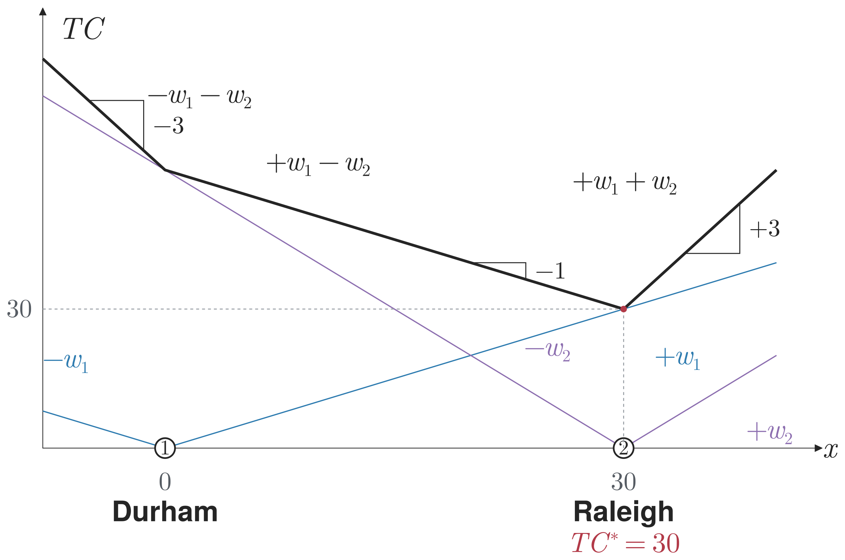
In Fig. 6, the darker line at the top is the total distance driven by the couple for each location x along US-70. It is labeled TC, total cost, since for this problem distance is the cost. A good way to visualize the total-cost curve is as the sum of each city’s weighted contribution. At its own city a trip covers no distance and adds nothing to the total; moving away from city i in either direction adds w_i per mile, so that city’s contribution is V-shaped, formed by lines of slope -w_i to the left of the city and w_i to the right. Summing the two contributions gives TC(x), which is piecewise-linear with a corner at each city, and between the cities its slope is w_1 - w_2 = -1, so TC falls all the way to Raleigh, where it reaches its minimum TC^\star = 30. There the slope changes from negative to positive, which is what marks Raleigh as the minimum.
At the fair point the two partners’ weighted travel is equal, 20 and 20, for a total of 40. At Raleigh the total drops to 30, its lowest possible value, but the Durham partner now bears all 30 while the Raleigh partner bears none. The difference, 40 against 30, is the price of fairness: equity costs the couple ten extra units of travel and buys an even split, while efficiency is cheaper and puts the whole burden on one partner. (Counting round trips doubles TC without changing the location decision.)
This coincidence, the fair point equalling the centroid, is exact only because there are two destinations, one equation in one unknown. With more destinations no single location can equalize everyone, and the two ideas separate into two problems that recur through Location: minimizing squared distance always gives the interior centroid, taken up in the later lecture on aggregate demand, while minimizing total weighted distance gives a weighted median that sits at a demand point, taken up in Sec. 4. The couple’s apartment selection problem is the seed of both.
Locating in Raleigh can in fact be the best of both worlds, but only once the objective is widened again. Concentrating the trips at Raleigh may let the couple keep one car instead of two, a saving with a clear dollar value. That saving does belong in the objective, and folding it in requires, as with the customer’s choice of beach, weighting the incommensurable together: once travel is evaluated at a shared rate, the miles and the cost of a car are both in dollars and can be added into a single total cost. Fairness is handled differently. Raleigh leaves the Durham partner bearing the whole commute, and rather than add that imbalance to the objective, the couple determines it outside the objective, through a compensating task such as cooking. The widened objective therefore minimizes total cost alone, with the car folded in and the even split arranged separately.
minimize: total weighted distance from the apartment to the two workplaces total couple cost: both partners’ travel valued at the couple’s single shared rate, plus the cost of the vehicles the couple keeps
solve for:
(a) location x of the apartment, any point along the corridor;
(b) whether the second car is kept, yes or no.
subject to:
(a) one-car: the second car can be given up only if the apartment is located in Raleigh, where the partner who works and studies there can walk
return: location x of the apartmentcouple’s plan: where to live, and whether to keep the second car
assumptions:
(a) apartment can be located anywhere along the corridor;
(b) Durham trip has weight 1 and the Raleigh trips have weight 2;
(c) couple pools its costs, so both partners’ travel is valued at the same rate, c dollars per mile, and the daily cost of a car is known;
(d) burdens can be rebalanced within the couple by compensating tasks, such as cooking, so any division of the total cost between the partners is achievable.
(e) couple coordinates fully, so a single objective can speak for both partners.
Model 7 is the first model in the course that will be carried past words into mathematics. Every model so far has been stated in words alone, its objective, constraints, and return values all in plain language, with several models in Lecture 1.3 descending straight to runnable Julia. A formulation sits between those two depths: the same model restated in symbols, changing nothing about what the model says. Restating a model in symbols is worth the effort because it forces a precision words cannot supply: a verbal description carries shades of meaning and can leave relationships implicit, while a formulation must name every quantity and pin down every relation exactly. That precision also makes the formulation the fixed reference across implementations. A model can be built in many vehicles, one programming language or another, each differing in its details, but the formulation is the same for all of them, a common specification an implementation can be checked against, so that discrepancies between what was meant and what was built are caught rather than buried in code. The translation is mechanical, and the callout’s own slots drive it. The quantities the model returns become decision variables, the unknowns the optimization is free to set, written under the \min operator; here they are the location x and the yes-or-no choice z. The given data receive symbols collected under where:, each traced to the assumption that supplies it. The objective in words becomes an expression in those symbols, and each constraint carries its letter and name over and becomes an equation or inequality the decision variables must satisfy. Model 7 also carries the course’s first subject to line, a good place to restate the distinction from Lecture 1.1: a constraint restricts the solution, ruling out answers the decision variables may not take (here, keeping the second car unless the apartment is in Raleigh), while an assumption restricts the world and its data, fixing what the model treats as given (that a car has a known daily cost, that the trips carry fixed weights).
One device in this formulation is worth singling out, because it recurs across all of operations research. A yes-or-no decision is encoded as a binary variable, a variable allowed only the values 0 and 1: here z = 1 means the second car is given up. Encoding the choice this way turns logic into algebra. The one-car condition “only if the apartment is in Raleigh” becomes the inequality a_2 z \le x, which permits z = 1 only once x has reached a_2, and the objective charges for the cars actually kept through the term c_v\,(2 - z).
\min_{x,\,z}\; C(x, z) \;=\; 2c\,\bigl( w_1\,\lvert x - a_1 \rvert + w_2\,\lvert x - a_2 \rvert \bigr) \;+\; c_v\,(2 - z)
subject to
\begin{aligned} a_2\,z &\le x &\quad& \text{(a) one-car: second car given up only if apartment in Raleigh}\\ z &\in \{0,1\} &\quad& \text{binary car choice} \end{aligned}
where
- x
- = apartment location along corridor (decision variable)
- z
- = \begin{cases} 1, & \text{if second car given up}\\ 0, & \text{if both cars kept}\end{cases}
- a_1
- = Durham’s position along corridor (miles)
- a_2
- = Raleigh’s position along corridor (miles)
- w_1
- = Durham’s daily trip weight (assumption (b))
- w_2
- = Raleigh’s daily trip weight (assumption (b))
- c
- = couple’s shared value of travel, dollars per mile (assumption (c))
- c_v
- = daily cost of one car.
One feature of the objective is worth pausing on. In the pure minisum model the distance could be counted one way, since doubling every trip to a round trip only scales the objective by a constant and moves neither the optimal location nor the fair split. Adding the car’s dollar cost ends that freedom: travel and the car must be measured in the same unit, dollars per day, so the travel term has to count the miles actually driven, the round trip there and back. A constant factor that is harmless in a single-term objective becomes essential once a second, differently scaled term joins it.
The bound a_1 \le x \le a_2 has deliberately been left out. Because total travel only grows as the apartment moves outside the two cities, no location beyond Durham or Raleigh could ever be optimal, so the bound would never bind and carries no information. A constraint that no optimal solution would violate can be dropped from the model, a simplification used often in linear and mixed-integer programming.
Working the formulation follows the same discipline as the beach comparison, each step resting on a named element of the model. For this couple, Durham sits at a_1 = 0 and Raleigh at a_2 = 30 miles. With both cars kept (z = 0), the daily cost between the cities is C(x, 0) = 2c(60 - x) + 2c_v, which falls all the way to Raleigh: the minisum pull of Model 6 is unchanged. At Raleigh, and only there, constraint (a) of Model 7 allows z = 1, dropping the second car: C(30, 1) = 60c + c_v. The fair location offers C(20, 0) = 80c + 2c_v by comparison, so Raleigh is cheaper by 20c + c_v every day, and assumption (d) keeps the choice fair: the compensating task rebalances the burden the location no longer shares. This is what the model’s name promises: the efficient location and an even settlement at once.
The lesson repeats the one from the beach. A location that looks inferior under a narrow objective can be the best choice once the objective is widened to include everything that actually matters (Model 7), provided the pieces are made commensurate so that a single objective can still be optimized. Choosing the objective, not solving it, is the hard and the important part of modeling a logistics problem.
What makes the widened objective legitimate turns on a word that has been doing quiet work all along: couple. A couple cooperates: it makes one decision and pays from one budget, which is what assumption (c) of Model 7 records when it evaluates both partners’ travel at the same rate c. The contrast is Model 3, where each customer valued a mile at a personal rate c and the market split, some customers choosing each beach; no single objective could speak for them all. One decision-maker with one rate is what allows two commutes to be added into a single objective at all.
Assumption (e) enters the model here, and its absence from Model 6 is worth a word. That model minimized total weighted distance, the miles the household drives; that sum is a physical quantity, well-defined however the partners split the driving, and an outside planner counting aggregate mileage would write the same objective, so it leans on nothing about who makes the decision. The widened model does three things the earlier one did not: it evaluates both partners’ travel at one rate (assumption (c)), it trades a kept car against miles driven (z), and it rebalances the leftover burden through a compensating task (assumption (d)). Each move treats the couple as a single economic unit, and assumption (e) is the justification for all three, the statement that one objective may stand for both partners. Cooperation was present in the earlier apartment models too, but idle; only here does the objective rest on it, so only here is it written down.
Cooperation also supplies the transfer that assumption (d) names. At the fair location, evenness was bought with ten extra weighted miles of driving a day, the price of fairness; the compensating task buys the same evenness for free. Equity has not been abandoned. It has moved out of the objective and into the settlement, and that move is available only because the decision-maker is a household rather than two strangers.
A firm is the couple at industrial scale. Its drivers’ miles are all valued at one rate not by agreement over dinner but by the wage: each driver is paid by the mile, so every mile, whoever drives it, costs the firm the same and is already compensated. The wage is assumption (d) institutionalized. That is why the claim that opened the lecture (Sec. 1) holds: in most private-industry problems transport cost really is proportional to distance, and the linear minisum objective is the right one, precisely because someone is being paid to do the driving. Two conditions are at work, not one: cooperation lets the separate travels be added into a single objective at all, and payment by the mile makes that objective linear. It is also why the cooperative branch of the taxonomy (Fig. 2) is the branch this course solves by summing costs. For travel on one’s own behalf, where no one pays by the mile, the nonlinear objectives of Sec. 5 take over.
One caution balances all of this. Every widening in the section, and the compensating task that let the couple have fair and cheap at once, assumed the parties cooperate fully, and that assumption is never exactly met, as even most couples, forever renegotiating whose turn it is to cook, can attest. A firm is not one mind but many self-interested agents, each with an agenda of their own, and the gap between the firm’s objective and theirs is the principal-agent problem. The subtle part is that centralizing does not close it: even a fully coordinated firm never reaches complete alignment, since aligning a team to the joint optimum is provably impossible in general and every hierarchy carries the residual frictions of bounded rationality and self-interest.8 So a model whose objective is defined for a perfectly cooperative firm can still miss what the firm actually does, because the people who carry it out are optimizing partly for themselves. This course does not try to close that gap: it takes the full coordination of assumption (e) of Model 7 as given throughout, an approximation its models make rather than a fact of the world, and asks only that it be remembered as such.
4. Solving the minisum problem by hand
Choosing the objective was the hard part of Sections 2 and 3; solving the one that results can be surprisingly easy. For the couple, the efficient (minisum) location was read straight off the corridor because there were only two destinations. This section finds the minisum location for any number of destinations, using nothing more than a sorted list and a running total: no computer, no calculus, and, remarkably, not even the distances between the facilities. It is the one class of location problem in this course that is genuinely solved by hand, which is why it is worth doing carefully; the Julia methods for the harder cases wait for the next lecture. The method, which puts the facility at the weighted median of the destinations, is stated as Model 8; the rest of the section solves it by hand.
minimize: total weighted distance from a new facility (NF) to the m existing facilities (EFs) along a line
solve for:
(a) location x of the NF, any point along the line.
subject to: none
return: location x^\star of the NF
assumptions:
(a) facilities lie on a single line, so distance is one-dimensional; a two-dimensional problem with rectilinear distance is solved by applying the model once along each axis;
(b) each EF’s weight w_i is known, and the EFs can be placed in order along the line, but their actual coordinates are not needed.
TC(x) = \sum_i w_i d_i = \sum_i \beta_i (x - a_i), \qquad \beta_i = \begin{cases} w_i, & \text{if } x \ge a_i \\ -w_i, & \text{if } x < a_i \end{cases} \tag{4}
where
- x
- = location of the NF along the line
- a_i
- = location of EF i along the line
- w_i
- = weight of EF i
- d_i
- = distance from the NF to EF i, \lvert x - a_i \rvert
- \beta_i
- = signed weight of EF i.
This means of finding the optimal solution only works because TC is linear; numerical optimization is needed otherwise.
algorithm minisum-1D;
{ input: m EFs on a line, EF i at position aᵢ with weight wᵢ > 0 }
{ output: index j of the weighted median; the NF locates there }
begin
order the EFs so that a₁ ≤ a₂ ≤ ⋯ ≤ aₘ;
W := Σᵢ wᵢ;
r := 0;
for j := 1 to m do
begin
r := r + wⱼ; { cumulative weight }
if r ≥ W/2 then return j; { weighted median found }
end;
end;Pseudocode, not Julia. The second formulation of Model 8 is pseudocode: a step-by-step statement of the method’s logic in no particular programming language. It is deliberately not Julia; stating the algorithm language-independently shows the logic itself, which any language could then implement, rather than tying it to one.
The facility the loop returns is the weighted median: the first EF at which the accumulated weight reaches half the total, \sum_{i=1}^{j} w_i \ge \frac{W}{2}. \tag{5}
Why does the median location correspond to the optimal location? From any EF location, take a small step of size \delta in either direction. Every EF behind the new facility becomes \delta farther away; every point ahead of it becomes \delta closer. The step is worth taking whenever more weight lies ahead than behind. Stepping toward the heavier side repeatedly, the process stops precisely when neither side holds more than half the total weight: the median location. That stopping condition is exactly the test in Eq. 5: at the first EF whose running total reaches W/2, the weight strictly behind is less than half, or an earlier EF would have been the first to reach it, and the weight strictly ahead is at most half, since the running total already accounts for the rest. Although it is unlikely, it is possible that the total reaches exactly W/2 at EF_j; in this case, a step in either direction trades equal weight against equal weight: every point from EF_j to the next unvisited facility EF_k is equally good, so the optimum is the whole interval between EF_j and EF_k rather than the single point at EF_j. In the objective function, this corresponds to a flat segment rather than a corner point.
A separate and more general result is the Majority Theorem: if any single EF holds at least half of the total weight, the NF goes there. The theorem is true for all minisum problems with metric distances, whatever the number of dimensions, so it is a property neither of the line nor of the median procedure, and it is worth applying as a first check before any other means of determining the location is tried.
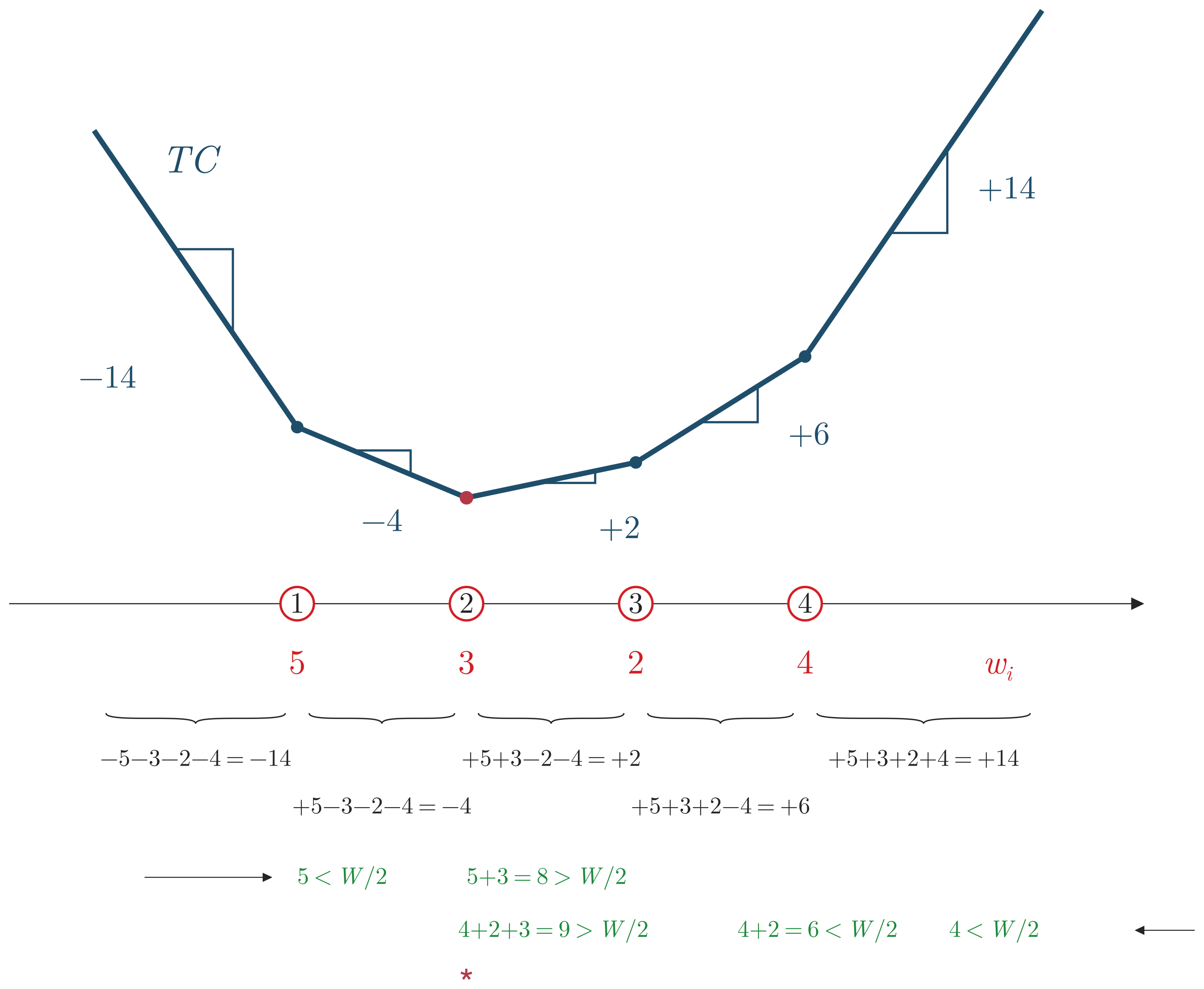
The reason the median location works can be seen in the total-cost curve (Fig. 7), whose net slope on each segment is the weight behind the location less the weight ahead of it. Each facility contributes a V-shaped weighted distance, and their sum is a piecewise-linear curve whose corners fall exactly at the existing facilities, so the lowest point is always one of them; there is never a reason to look between the facilities. It is also why only the order of the facilities matters, not their coordinates: the procedure never measures a distance, it only sorts the facilities and adds weights until half the total is reached. One consequence is worth pausing on. Because a coordinate is never used, the answer is completely insensitive to how far away a facility sits. Take the westernmost city in the example below and move it from the mountains all the way to Nashville, or to California; as long as its weight is unchanged and it stays the westernmost, the optimal location does not shift at all.
The procedure is easiest to see on a real corridor.
Example 1: Minisum location along I-40
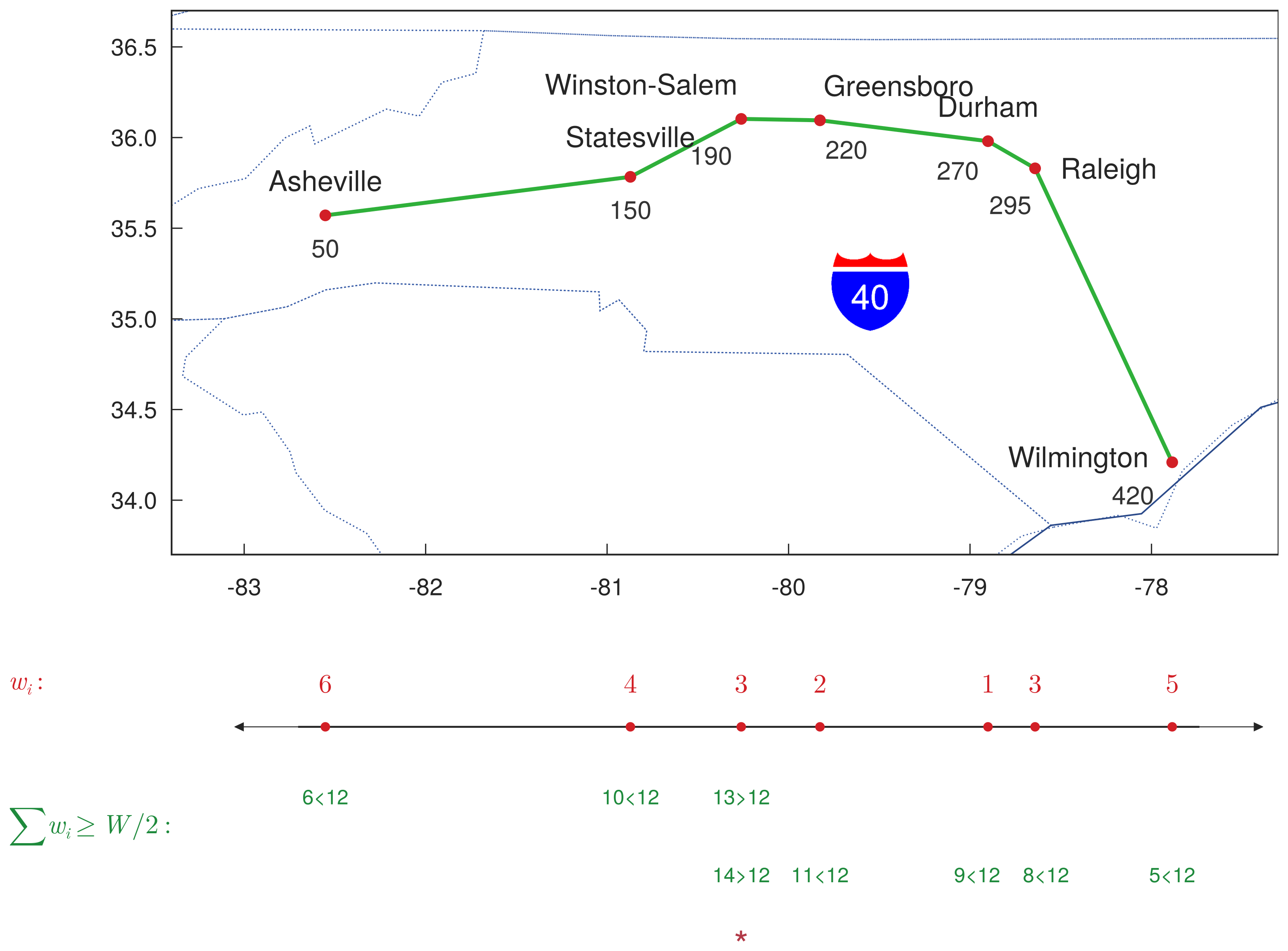
A company will build a single facility along I-40 to serve customers in seven North Carolina cities (Fig. 8). The weekly demand, in truckloads, is 6, 4, 3, 2, 1, 3, and 5 for Asheville, Statesville, Winston-Salem, Greensboro, Durham, Raleigh, and Wilmington. Determine the minisum location, first from the cities in geographic order and then from the same data listed out of order.
Example 1(a): Cities in geographic order
With the cities already ordered west to east, apply the median procedure of Model 8.
The total weight is W = 6+4+3+2+1+3+5 = 24, so the target is W/2 = 12. The lower panel of Fig. 8 carries out the search directly on the ordered corridor: the weights are accumulated city by city until the running total first reaches W/2, which happens at Winston-Salem. The figure runs that count from both directions at once, west to east and east to west, and the two converge on the same city. That convergence is the point worth holding onto: the median does not depend on which end the accumulation starts from, so the count can be made from whichever end is more convenient, and the two directions meeting at the same facility is a built-in check that the ordering and the arithmetic are right.
Winston-Salem, the first city whose cumulative weight reaches W/2 = 12.
The mile markers on Fig. 8 were never used, only the ordering. The next part shows why getting that ordering right is the one step that cannot be skipped.
Example 1(b): Data given out of order
The trip counts for five cities are given in alphabetical order: Asheville 5, Durham 15, Greensboro 10, Statesville 10, and Wilmington 20. Determine the minisum location.
Alphabetical order is not order along the road. West to east the five cities run Asheville, Statesville, Greensboro, Durham, Wilmington, so the weights must be resequenced before a running total means anything. With W = 60 and W/2 = 30, accumulating in the correct order (5, 15, 25, 40) reaches 30 at Durham. Accumulating in the alphabetical order as given (5, 20, 30) would instead stop at Greensboro, the wrong city; the trap is applying the procedure before sorting.
Durham, once the cities are in geographic order. Summing the alphabetical list as given gives the wrong answer, Greensboro.
The same procedure reaches into two dimensions whenever distance is measured rectilinearly, as the sum of the horizontal and vertical displacements rather than the straight-line distance. Rectilinear distance is the natural model inside a facility, where a worker moving between departments follows the aisles and turns at right angles instead of cutting across the floor. Because a rectilinear distance is the sum of an x-distance and a y-distance, the two axes do not interact, and the two-dimensional problem separates into two independent one-dimensional problems: solve for the best x by the median procedure, solve for the best y the same way, and combine the two.
Example 2: Snack machine on a factory floor
A snack machine will be placed on a factory floor to serve eight departments (Fig. 9). The number of trips per shift is 19, 53, 82, 42, 9, 8, 39, and 6 for departments 1 through 8, located at (5,70), (70,95), (5,25), (15,60), (60,95), (15,25), (60,15), and (90,60). Assuming rectilinear travel, determine the minisum location.
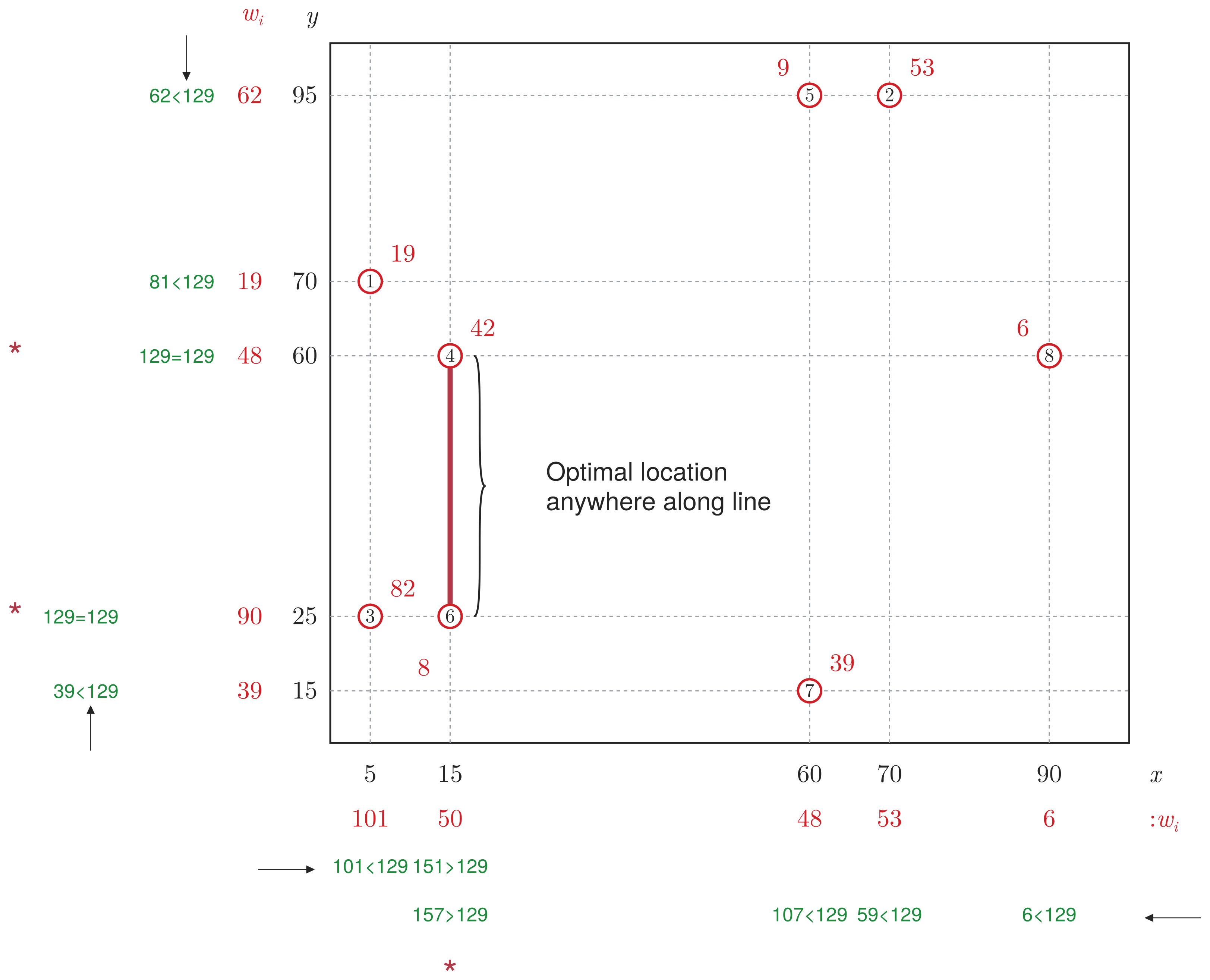
The total weight is W = 258, so each axis looks for a running total of W/2 = 129. The two searches are read off the margins of Fig. 9, just as on the one-dimensional corridor, with one wrinkle: departments sharing a coordinate combine their weights before the count. The x-search settles on the single value x = 15, where the weight on one side of the split outweighs the other.
The y-search is the case worth dwelling on, because its answer is not a coordinate but a line segment. Counting up from the bottom, the cumulative weight reaches W/2 exactly at y = 25; counting down from the top, it reaches W/2 exactly at y = 60. Neither coordinate alone is the answer: every point between them is equally optimal, and Fig. 9 marks this stretch with a brace labeled optimal location anywhere along line. This is the tie case of Model 8, and it arises whenever the weight divides into two exactly equal halves. Why the entire segment ties is worth seeing directly: sliding the machine up the segment moves it away from the 129 units of weight at or below y = 25 and an equal 129 units toward the weight at or above y = 60, so the two changes cancel and the total travel does not move. Only when one side outweighs the other, as on the x-axis, is the optimum pinned to a single facility. The freedom is genuine rather than a rounding artifact: any point on the segment is equally good for travel, so a second criterion, such as where the floor is clear, can determine where the machine actually goes.
x^\star = 15, a single value; y^\star anywhere from 25 to 60. Any point on that vertical segment minimizes the total rectilinear travel.
The rectilinear method is useful even when the true distances are not rectilinear at all, but great-circle distances across the curved surface of the earth, as long as only a rough location is needed.
Example 3: Great-circle approximation
A distribution center will serve six customers, shipping 25, 42, 24, 10, 24, and 11 truckloads per year to Raleigh, NC; Atlanta, GA; Louisville, KY; Greenville, SC; Richmond, VA; and Savannah, GA, at (36°N, 79°W), (34°N, 84°W), (38°N, 86°W), (35°N, 82°W), (38°N, 77°W), and (32°N, 81°W). Find an approximate minisum location by treating latitude and longitude as rectilinear coordinates.
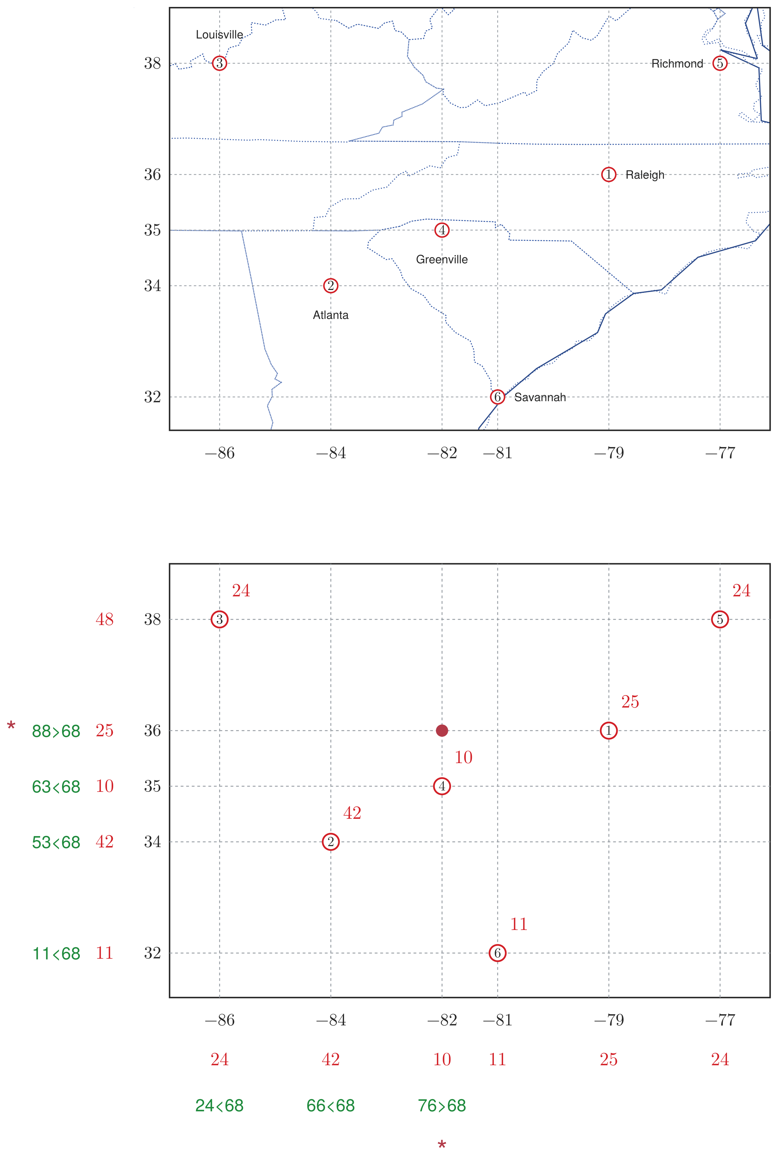
Latitude and longitude are angles, not miles, so a “distance” built from them is not a physical distance; but the median procedure never uses distances, only the ordering along each axis, which latitude and longitude supply perfectly well. Applying the one-dimensional procedure to the six latitudes (W = 136, W/2 = 68) lands on 36°N, and again to the six longitudes on 82°W (Fig. 10). The facility goes at (36°N, 82°W), Raleigh’s latitude and Greenville’s longitude, not necessarily a real city, since the two axes are solved independently.
(36°N, 82°W), from the median latitude and the median longitude taken separately.
Crude as it looks, the approximation is good, though only for its era: fifty years ago, with computers not readily available and no easy alternative at hand, a location gotten by hand and within about 65 miles of the true great-circle optimum would have served well. What is striking is that there is little evidence anyone actually used it.
5. Other location objectives
The minisum problem of Section 4 is the linear, hand-solvable case: cost proportional to distance, an objective a sort and a running total dispose of. Most other objectives are nonlinear, cost growing faster or slower than distance, and they generally require a computer. This section surveys the ones worth knowing and connects them back to the couple of Section 3.
Cost is proportional to distance whenever whoever does the travelling is paid by the mile, as a hired truck driver is, and then the linear minisum objective is exactly right. For people travelling on their own behalf it usually is not: a long trip carries a psychological cost out of proportion to its length, the same reason most people would rather make several short drives than one long one. A well-known regularity, Marchetti’s constant, captures the effect from the other side: the average commute has stayed at about one hour a day across widely different eras.9 It is why cities grew only as large as their transport allowed. When everyone walked, a city reached about as far as a half-hour walk each way; horse-drawn trolleys let it spread further, and the automobile further still, each technology enlarging the one-hour reach rather than changing the hour. A technology that lowers the felt cost of travel, such as a self-driving car in which the commute becomes usable time, would be expected to expand cities again.
The couple of Section 3 was already an instance of this. Their fair location, the centroid that equalized the two partners’ travel, is the point that minimizes the sum of squared distances, and squaring the distance is precisely a nonlinear objective: it penalizes a long trip more than proportionally, which is another way of evaluating the psychological cost of a lopsided commute. Seen this way, equity and psychological cost are the same departure from the linear minisum, and the fair centroid is location theory’s simplest nonlinear objective.
Two further nonlinear objectives change not how distance is valued but how the individual facilities’ costs are aggregated: instead of summing them, take the largest, or the smallest.
minimize: largest distance from the new facility to any existing facility
solve for:
(a) location of the new facility, any point in the plane.
subject to: none
return: location of the new facility
assumptions:
(a) what matters is the worst case, not the total or the average.
maximize: smallest distance from the new facility to any existing facility
solve for:
(a) location of the new facility, any point in the plane.
subject to: none
return: location of the new facility
assumptions:
(a) facility is undesirable, so the aim is to stay as far as possible from the nearest existing facility;
(b) facility is confined to a bounded region, without which the problem has no finite answer.
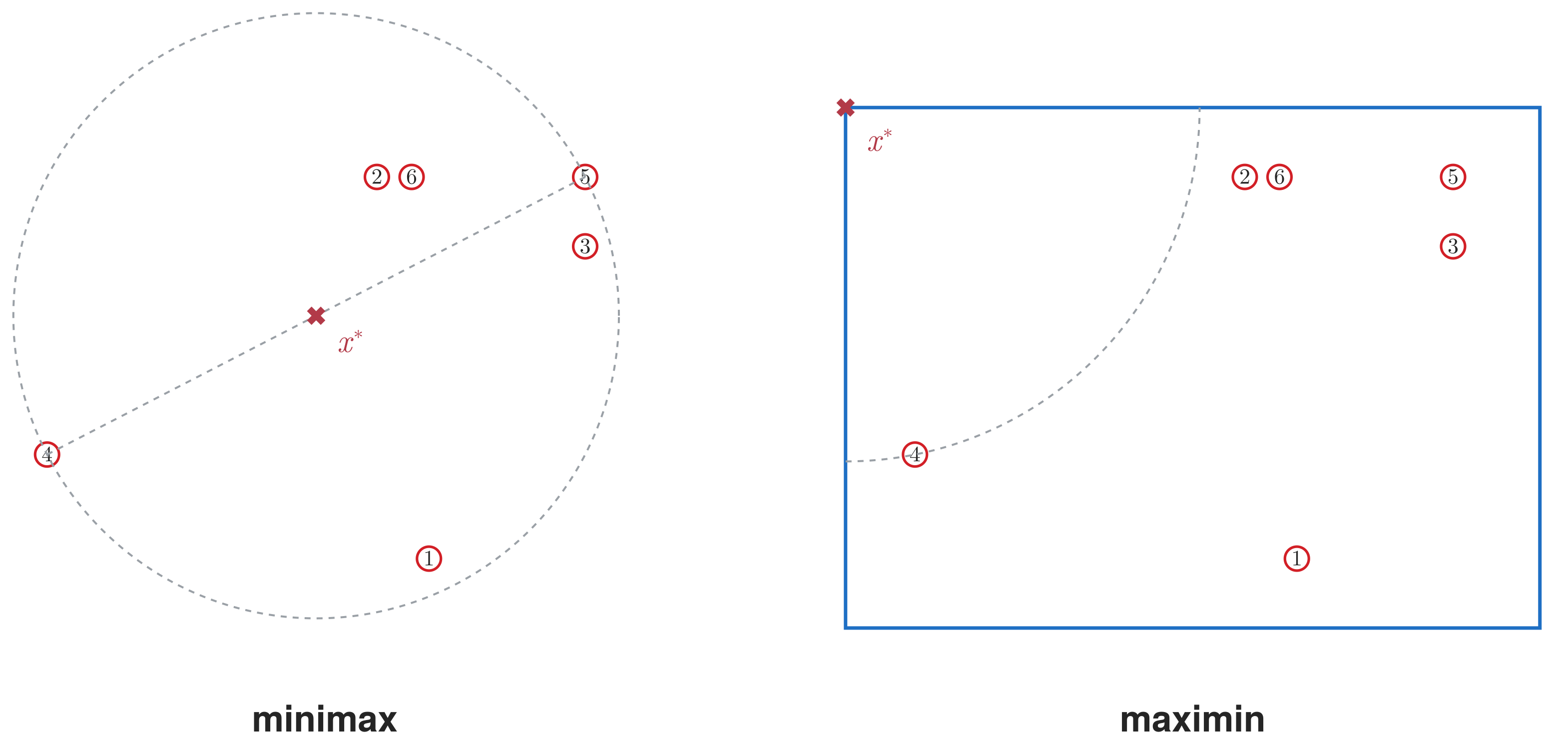
Both objectives are drawn for the same six facilities in Fig. 11. The minimax objective (Model 9) fits a facility whose cost is dominated by its worst case rather than its total, such as a fire station: what matters is the longest response, since the difference between reaching a fire in five minutes and ten is the difference between saving and losing the structure, while the difference between five and six minutes hardly matters.
The maximin objective (Model 10) is its mirror image, used to place an obnoxious facility that everyone wants to be far from, such as a waste-treatment plant. On its own that problem is ill-posed, since the facility would run off to infinity; it makes sense only inside a bounded region. A county siting a waste facility, for instance, placed it right against the neighboring county’s line, as far as it could get from its own residents.
6. A taxonomy of objectives
The lecture began by sorting location problems by their objective (Fig. 2); it can end by sorting the objective functions themselves (Table 1). Writing d_i for the distance from the new facility to existing facility i, every problem considered here minimizes the linear minisum objective or one of its nonlinear relatives. The linear form is the workhorse, cost proportional to distance and the easiest to solve; the nonlinear forms arise when cost is not proportional to distance, and generally require a computer.
| Type | Name | Objective | Where treated |
|---|---|---|---|
| Linear | minisum | \min \sum_i w_i d_i | Sec. 1, 4; 2.2 Sec. 3 |
| Nonlinear | center of gravity | \min \sum_i w_i d_i^2 | Sec. 3 |
| minimax | \min\{\max_i d_i\} | Sec. 5; 2.2 Sec. 4 | |
| maximin | \max\{\min_i d_i\} | Sec. 5; 2.2 Sec. 4 | |
| fixed cost (affine) | \min \sum_i (k_i + w_i d_i) | later lecture | |
| economy of scale | \min \sum_i w_i \sqrt{d_i} | not covered |
Three of the five nonlinear forms have appeared in this lecture: the center of gravity of Sec. 3, and the minimax and maximin of Sec. 5. The fixed-cost form, which adds a fixed charge k_i for using a facility to the linear travel cost, is the one nonlinear case this course solves, taken up with discrete location in a later lecture. The last, economy of scale, is listed only to mark the range: where squaring the distance penalizes a long trip more than proportionally, the square root does the opposite, its cost growing slower than distance. Choosing among these objectives, not solving any one, remains the modeling decision the lecture has been about.
Endnotes
R. L. Ackoff, Redesigning the Future: A Systems Approach to Societal Problems (New York: John Wiley & Sons, 1974), 8.↩︎
Base geography (coastline, state boundaries, Great Lakes) is from Natural Earth via GeoMakie (public domain); the Appalachian ridge, the fall line, and the river courses are drawn schematically to highlight the features named in the text.↩︎
Before Raleigh, the General Assembly had no permanent home, meeting in turn at New Bern, Hillsborough, Fayetteville, and Tarboro. In 1788 a convention resolved to fix the seat of government centrally, within ten miles of Isaac Hunter’s plantation in Wake County, with Fayetteville the chief rival; rather than adopt an existing town, commissioners laid out a new capital there on land bought from Joel Lane in 1792. “Capitals, Colonial and State,” NCpedia (State Library of North Carolina), https://www.ncpedia.org/capitals-colonial-and-state (accessed July 2026).↩︎
This point is drawn from a comment by Sean March, Fall 2020.↩︎
Harold Hotelling, “Stability in Competition,” The Economic Journal 39, no. 153 (1929): 41–57.↩︎
Harold Hotelling, biography, MacTutor History of Mathematics Archive, University of St Andrews, https://mathshistory.st-andrews.ac.uk/Biographies/Hotelling/ (accessed July 2026).↩︎
NC State University, Department of Statistics, “History,” https://statistics.sciences.ncsu.edu/know-us/history/ (accessed July 2026).↩︎
That full alignment is unattainable even in principle, not merely a failure to centralize, is a formal result: B. Holmström, “Moral Hazard in Teams,” Bell Journal of Economics 13, no. 2 (1982): 324–340, shows that a team dividing its own output among its members cannot make the joint optimum a self-enforcing equilibrium (the free-rider problem).↩︎
The city-size framing follows B. Potter, “How the Car Came to LA,” Construction Physics, https://www.construction-physics.com/p/how-the-car-came-to-la (accessed July 2026), which applies Marchetti’s constant to urban form. On the constant itself: C. Marchetti, “Anthropological Invariants in Travel Behavior,” Technological Forecasting and Social Change 47, no. 1 (1994): 75–88; the one-hour/day figure is Y. Zahavi’s, which Marchetti frames as a stable invariant.↩︎