Optim is a pure-Julia library for numerical optimization: it minimizes a user-supplied objective function, with both derivative-free methods (Nelder-Mead) and gradient-based methods (quasi-Newton such as BFGS). It is the general-purpose optimizer of the Julia ecosystem, not specific to logistics.
GeoMakie is the geospatial extension of the Makie plotting ecosystem: it adds map projections and reference geography, such as coastlines and political boundaries from the Natural Earth dataset, so that data given in longitude and latitude is drawn on a correctly projected map rather than on a plain Cartesian axis.
New Logjam functions used
aligntext: Determines text alignment and offset positions for given points.
d1: Calculate rectilinear (Manhattan, L₁) distance between two points.
d2: Calculate Euclidean (L₂) distance between two points.
dgc: Calculate the great circle distance between two points.
dists: Compute distance matrix between two point sets using specified metric.
lonlat2loc: Find nearest place to a (lon, lat) coordinate pair (reverse geocoding).
makemap: Creates map visualization for predefined or user-defined region of interest.
prt: Pretty-print a matrix, vector, or DataFrame with smart formatting.
st2fips: Convert a two-character symbol for US states and territories to its corresponding FIPS code.
usplace: Returns DataFrame containing U.S. place data.
wcentroid: Weighted geographic centroid of points (LON, LAT) with weights w, corrected for longitude convergence toward the poles by a cos(lat) factor.
Companion script
2-loc-2.jl, runnable Julia extracted from this lecture’s code blocks.
Lecture 2.1 sorted location problems by their objective and solved the linear minisum objective by hand, in one dimension and in two dimensions under rectilinear distance. It left two questions open. First, where do the weights w_i in the minisum objective come from? Second, how is the location found when the problem is not one dimensional and the distances are not rectilinear, so that the by-hand median procedure no longer applies? Secs. 1 and 2 describe how the weights are determined and Sec. 3 describes a general-purpose numerical procedure that can be used to determine locations.
1. Weights: monetary vs physical
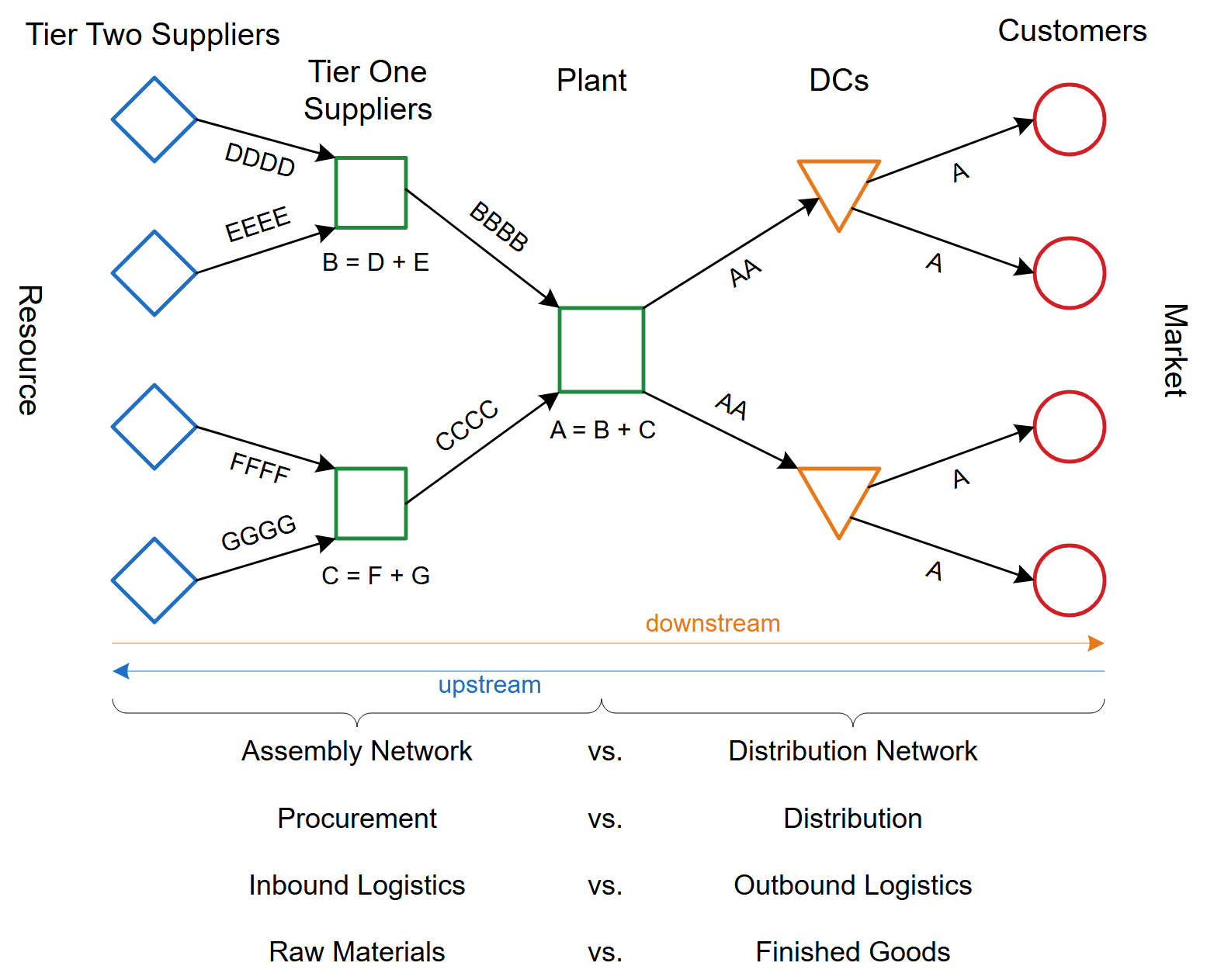
Fig. 1 shows a typical supply chain for a single plant. In the figure, items D and E provided by two different tier-two suppliers are shipped to a tier-one supplier where they are used to produce item B, units of which are then shipped to the plant. Similarly, items F and G are used to produce item C, which, along with B, are the two raw materials used to produce the finished good A. Units of A are shipped to distribution centers (DCs), from which they are delivered to the final customer. The number of units shown along each lane (or arc) in the figure is meant to indicate the typical size of each shipment; e.g., one of the reasons that a DC might be used is that it is cheaper to transport larger loads from the plant to the DC and then transport small loads to each customer as needed.
Figure 1: Typical logistics network for a plant.
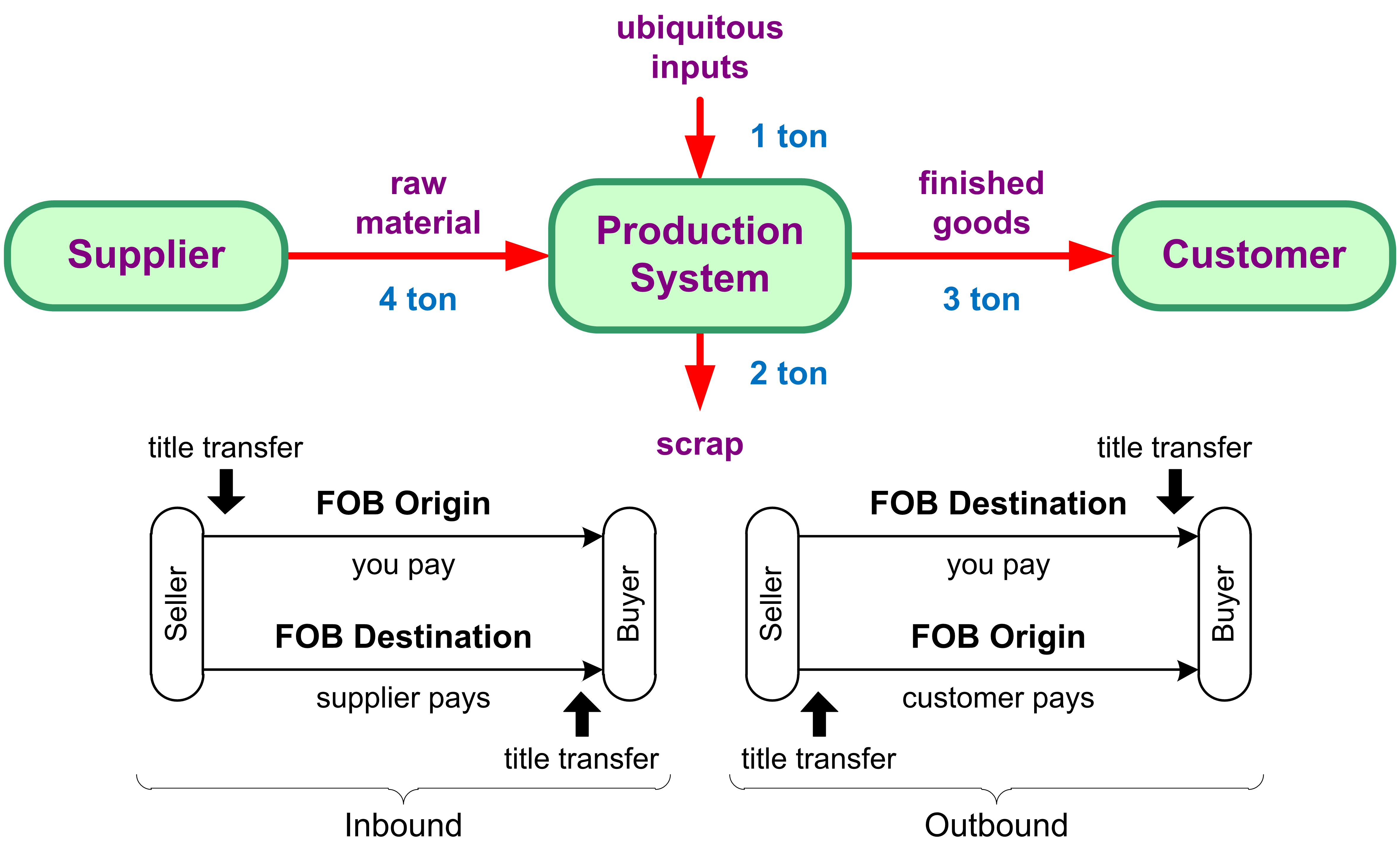
As shown in Fig. 2, a production system can be considered as a node (or facility) in a logistics network that converts raw materials procured from suppliers into finished goods that are distributed to customers. For most production systems, the material input to the system equals the material output from the system. Raw materials are those inputs that are transported to the production facility; ubiquitous inputs (e.g., water) are those available at any location, so that they do not need to be transported. Finished products are those outputs transported from the facility; while scrap is the output that is disposed of locally (although some outputs termed “scrap” are sometimes transported long distances from the facility for disposal or rework).
Figure 2: Top: the basic production system. Bottom: the corresponding FOB terms, inbound and outbound.
The bottom portion of Fig. 2 illustrates two different shipping terms that describe when the transfer of title occurs when goods are transported from the seller to the buyer: FOB Origin and FOB Destination, where FOB stands for free on board.1 In most cases, the cost of transporting the goods is paid for by whoever is the owner of the goods during the transport. Taking the production system as the buyer, the supplier (the seller) would pay for the transport of goods from the supplier’s location (the origin) to the production facility (the destination) if the shipping terms were FOB Destination.
The choice of FOB terms does not usually affect the location decision at all; it only fixes who pays for the freight. If a purchaser pays for the transport (FOB Origin), then they would typically pay less than they would if the supplier paid for the transport (FOB Destination). As a result, the sum of the transport cost and the purchase cost is unaffected by the FOB terms, and therefore does not impact the location decision. What typically determines who pays for the transport is who can provide the transport at lower cost. A large retailer with an extensive logistics network and its own fleet of trucks will typically be able to provide the transport at a lesser cost compared to a small supplier. The saving that the lower cost creates is then allocated between the parties by bargaining.
The conclusion that FOB terms do not affect the location rests on the market being competitive. A producer with a strict monopoly could locate for its own convenience and still make the sale. With competitors along I-40 producing the same product, a customer buys from whoever delivers at the lower price, so a plant placed far from its customers loses them to a nearer rival: Hotelling’s law from Lecture 2.1, in the market rather than on the sand.
Behind the choice of terms sits a short chain of cost definitions that lead to transport cost, which is the cost most impacted by the location decision. Procurement cost is the landed cost at the supplier plus the inbound transport cost. Adding the local resource cost, meaning labor and whatever materials are bought locally, gives the production cost; adding the outbound transport cost to that gives the total delivered cost. The transport cost, TC, is the sum of the inbound and the outbound transport costs alone:
\begin{aligned}
\text{procurement cost} &= \text{landed cost at supplier} + \text{inbound transport cost}\\
\text{production cost} &= \text{procurement cost} + \text{local resource cost}\\
\text{total delivered cost} &= \text{production cost} + \text{outbound transport cost}\\
\text{transport cost} &= \text{inbound transport cost} + \text{outbound transport cost}
\end{aligned}
\tag{1}
For most location problems only that last quantity is of interest, and everything else is assumed, as a first approximation, not to change with location.
The TC(X) minimized in Eq. 2 below is exactly the last line of Eq. 1. Assuming that local input costs are either the same at every location or are insignificant as compared to transport costs, the minisum transport-oriented single-facility location problem is to locate a new facility (NF) to minimize the sum of weighted distances between NF and m existing facilities EF_i,i = 1, \ldots, m:
=physical weight (tons), or f_i (physical weight rate, tons/year)
r_i
=transport rate ($/ton-mile)
d(X, P_i)
=distance between NF at X and EF_i at P_i (miles)
c_i
=unit cost ($/ton), used to determine q_i after NF located
X
=location of new facility (NF)
P_i
=location of existing facility i (EF_i)
m
=number of EFs.
Determining q_i once the NF is located is a transportation problem. The quantity that drives the location is the monetary weight, and it is worth splitting into two parts. The physical weight is the easy one, tons per year. Multiplying it by the transport rate, in dollars per ton-mile, cancels the tons and leaves a rate in dollars per mile per year: the monetary weight. In practice people drop the qualifier and simply say “the weight,” always meaning this monetary one.
If the physical weight q_i is used, then TC in Eq. 2 is in units of $; if, instead, the physical weight rate f_i in units of tons per year is used, then TC is in units of $/year.
An activity is weight-gaining when its outbound monetary weight exceeds its inbound, and weight-losing in the reverse. The distribution center is the standard weight-gaining case: cases of a product arrive on a tractor-trailer and leave on a smaller delivery truck whose cost per ton-mile might be twice as high, so the transport rate, and with it the monetary weight, roughly doubles even though the product itself has not changed.
When the same vehicles carry the inbound and outbound flows, one transport rate is common to every term. Taking it as one turns the objective into minimizing total distance, so the minimum-cost problem becomes a minimum-distance problem, solved by the same median procedure as in Model 8 in Lecture 2.1. The transport rate has to be included explicitly only when the flows travel at different costs.
That objective is the total transport distance TD, in miles per year:
Setting the transport rate r_i = 1 leaves the monetary weight w_i as f_i, the trips per year, and d(X, P_i) as the per-trip distance in miles per trip, so trips per year times miles per trip gives miles per year.
2. Procurement and distribution
A plant draws raw materials from its suppliers and ships finished goods to its customers, so its location is pulled from both sides at once: procurement, the inbound flows, and distribution, the outbound flows. Each existing facility, supplier or customer, enters the minisum objective of Eq. 2 through its monetary weight, and the location balances all of them together.
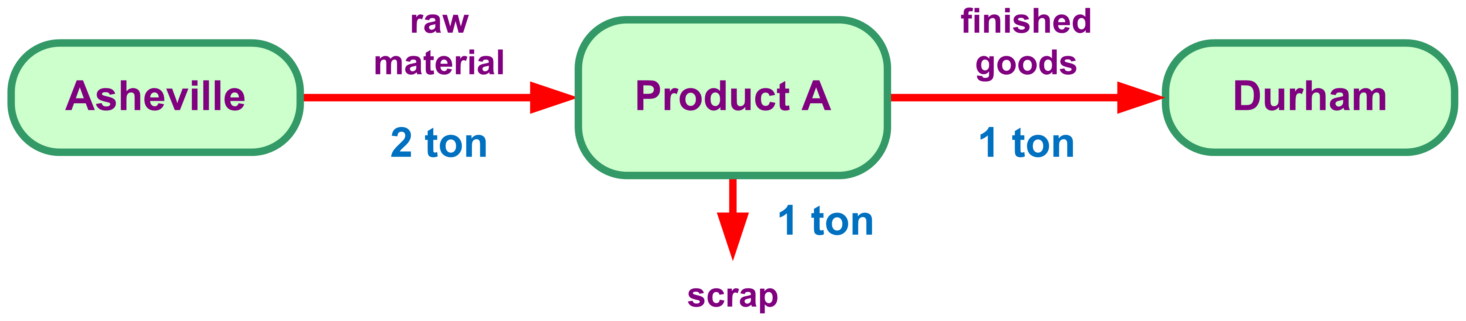
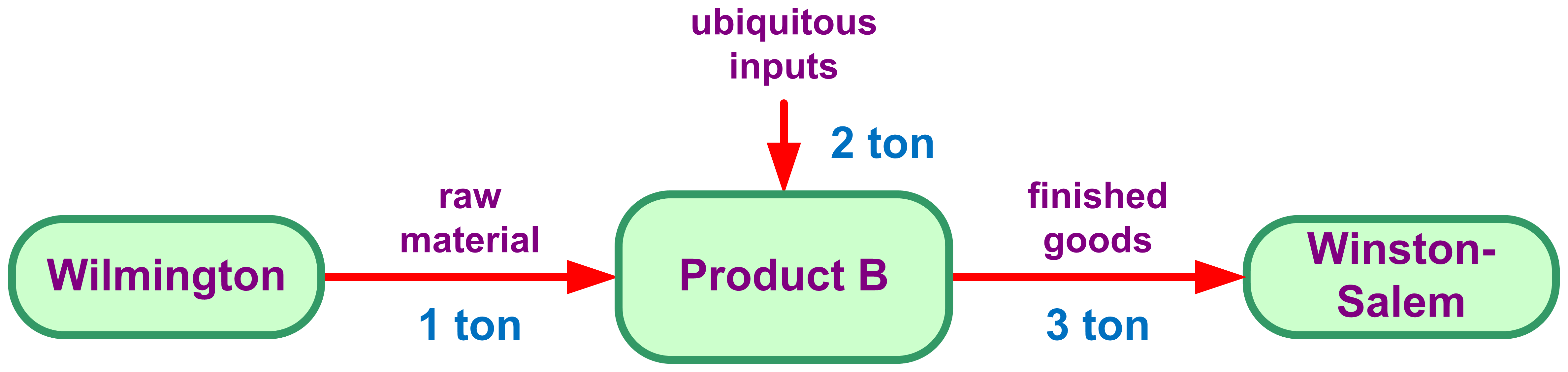
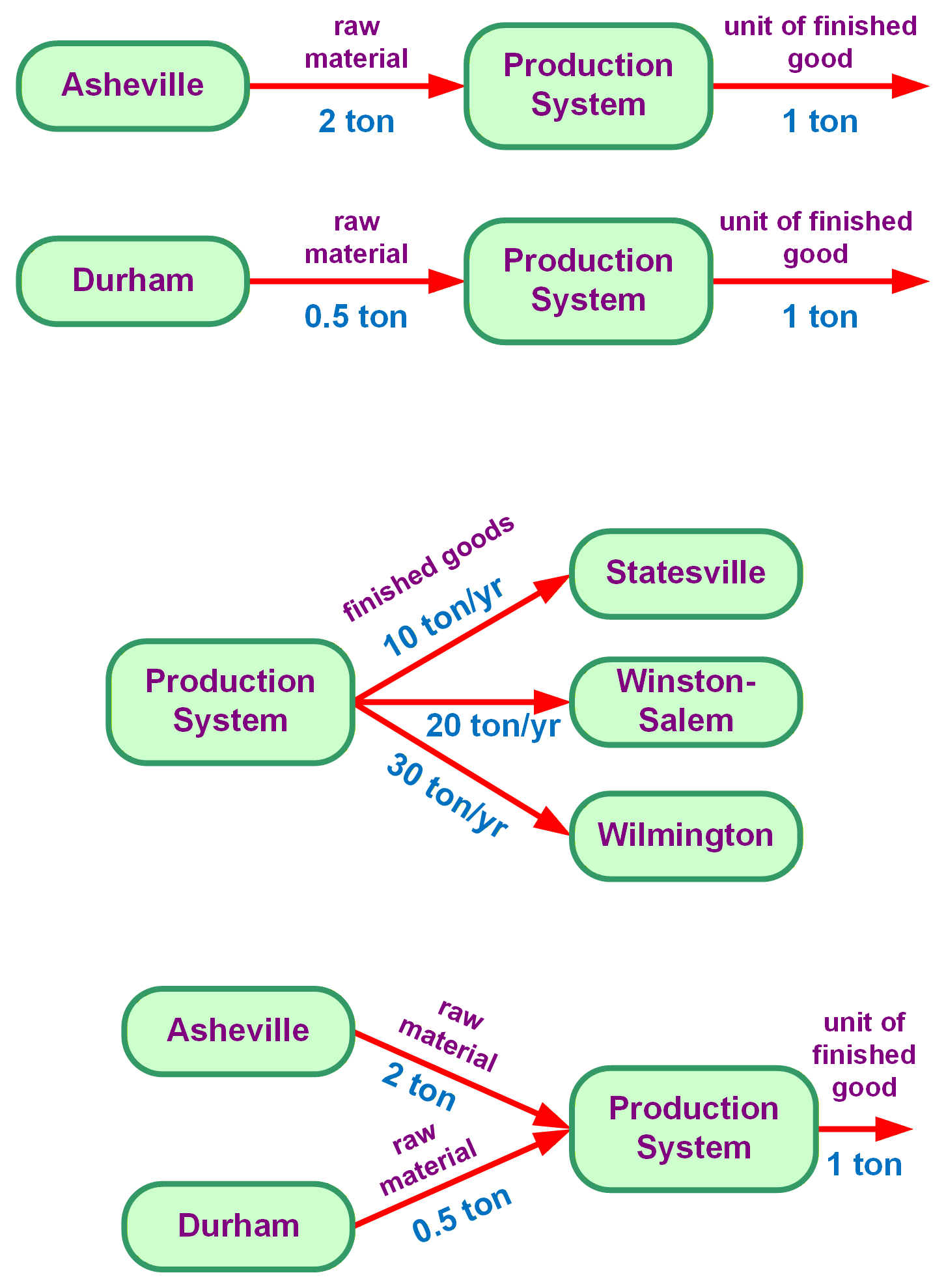
The simplest case, one supplier and one customer, already shows how the weights determine the location. Two products illustrate the two extremes (Fig. 3 and Fig. 4), with the same transport rate on both sides, so only the physical weights matter.
Figure 3: Product A: two tons of raw material from Asheville yield one ton of finished goods for Durham, with one ton of scrap disposed of locally.
Figure 4: Product B: one ton of raw material from Wilmington, plus two tons of ubiquitous inputs, yield three tons of finished goods for Winston-Salem.
Product A is physically weight-losing: two tons move in for every one ton that moves out, so every mile the plant sits closer to Asheville saves a net ton-mile of transport, and the plant belongs at the supplier. Product B is weight-gaining: its ubiquitous inputs, such as water or air, are available everywhere and incur no transport, so only one ton moves in for every three tons that move out, and the plant belongs at the customer. If the two products were made in a single shared plant, neither answer stands alone: the location would depend on how much of each product is made, so each product’s annual demand f_i enters, and the problem becomes exactly the weighted minisum of Eq. 2.
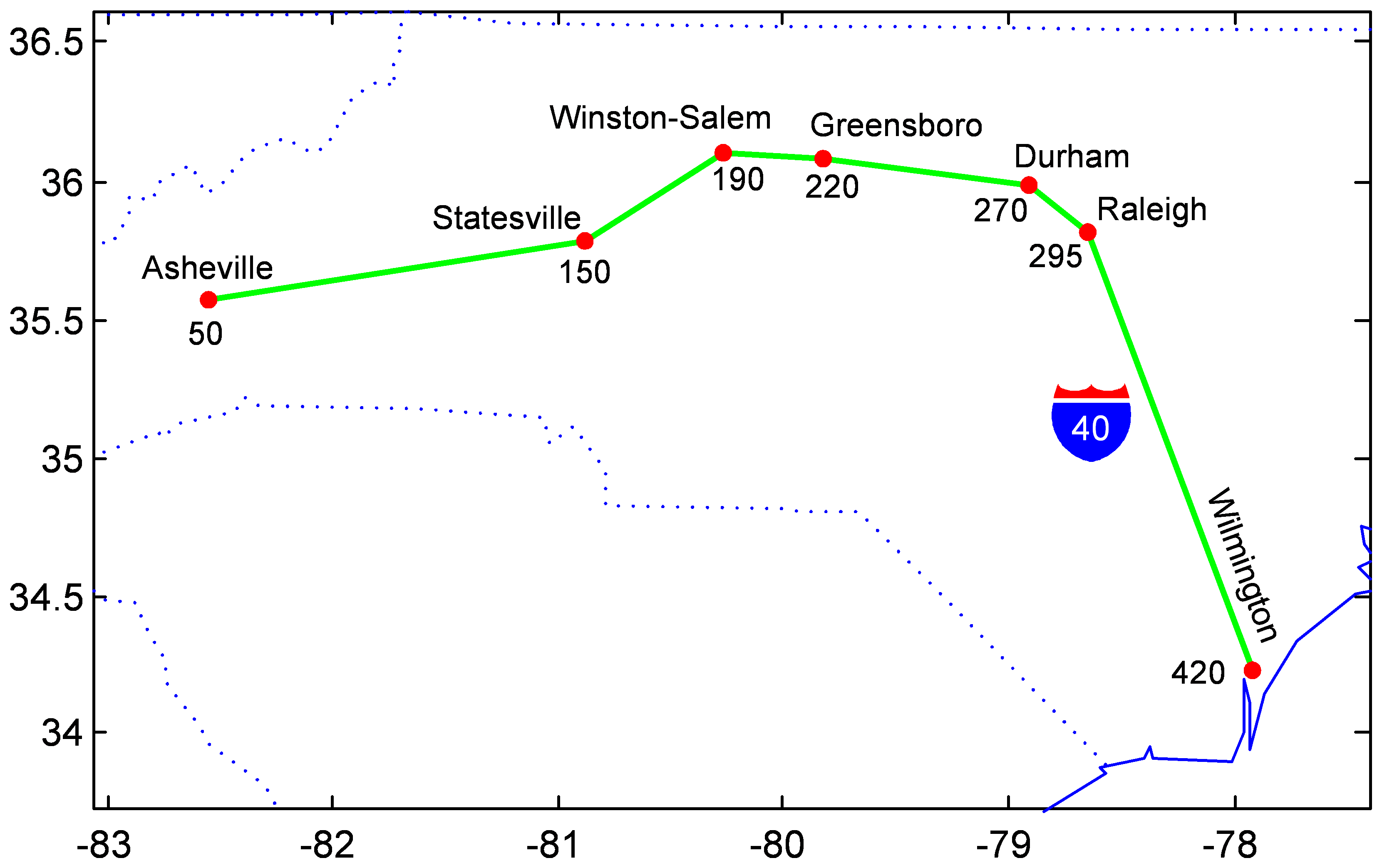
The worked example combines both sides at full scale: a plant on the I-40 corridor (Fig. 5) with two suppliers, three customers, and different inbound and outbound transport rates.
Figure 5: The I-40 corridor with mile markers: Asheville (50), Statesville (150), Winston-Salem (190), Greensboro (220), Durham (270), Raleigh (295), and Wilmington (420).
Example 1: Plant location along I-40
A product is to be produced in a plant located along I-40. Two tons of raw materials from a supplier in Asheville and a half ton of a raw material from a supplier in Durham are used to produce each ton of finished product that is shipped to customers in Statesville, Winston-Salem, and Wilmington. The demand of these customers is 10, 20, and 30 tons per year, respectively. Raw materials cost $0.33 per ton-mile to ship to the plant; finished goods cost $1.00 per ton-mile to ship from the plant. All scrap is disposed of locally. Determine where the plant should be located so that procurement and distribution costs (i.e., the transportation costs to and from the plant) are minimized, and whether the plant is weight-gaining or weight-losing.
Example 1(a): From the bill of material to the monetary weights
Determine each existing facility’s monetary weight, outbound from the demands and inbound through the bill of material.
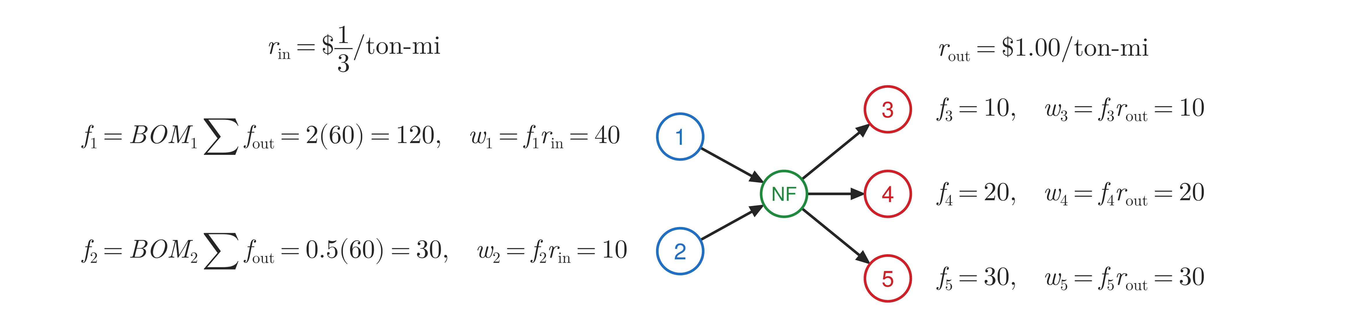
The outbound side comes first, because the customers’ demands are given directly: each customer’s monetary weight is its demand times the outbound rate. The inbound side follows from the bill of material (Fig. 6): the customers together take \sum_i f_i = 60 tons of finished product per year, so the plant must pull in two tons of Asheville material and half a ton of Durham material for each of those tons, and each supplier’s monetary weight is that physical flow times the inbound rate (Fig. 7).
Figure 6: Per ton of finished product, the plant consumes two tons of raw material from Asheville and half a ton from Durham.
Figure 7: Computing the five monetary weights. Each row sits at its facility’s height: suppliers 1 and 2 on the left, their physical flows following from the bill of material and evaluated at the inbound rate; customers 3, 4 and 5 on the right, their demands evaluated at the outbound rate. Code block 1 below carries out exactly these calculations.
# Code block 1: monetary weights from flows and ratesfout = [10, 20, 30] # ton/yr to the three customersrout =1.00# $/ton-mi outboundwout = fout .* rout # customer monetary weightsBOM = [2.0, 0.5] # ton raw per ton out: Ashvl, Durhamfin = BOM .*sum(fout) # inbound physical flows (ton/yr)rin =1/3# $/ton-mi inbound, stated as $0.33win = fin .* rin # supplier monetary weights@show wout fin win;
The five monetary weights, in dollars per mile of plant movement, are 40 (Asheville), 10 (Statesville), 20 (Winston-Salem), 10 (Durham), and 30 (Wilmington). The suppliers’ weights land on the same footing as the customers’, so from here the problem no longer cares which facilities ship in and which ship out.
Example 1(b): Locating the plant
Order the facilities along I-40 and apply the median procedure of Model 8 in Lecture 2.1.
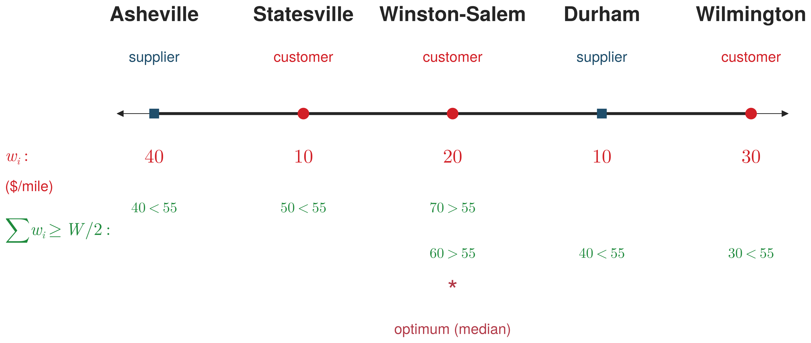
With every weight known, the corridor is one-dimensional and the median procedure applies unchanged: sweep west to east, accumulate weight, and stop at the first facility where the running total reaches half the grand total.
# Code block 2: west-to-east order and the weighted mediancity = ["Asheville", "Statesville", "Winston-Salem","Durham", "Wilmington"] # west-to-east orderw = [win[1], wout[1], wout[2], win[2], wout[3]] # $/mi, W to EW =sum(w)@show W W/2cumsum(w)city[findfirst(>=(W /2), cumsum(w))]
W = 110.0
W / 2 = 55.0
cumsum(w) = [40.0, 50.0, 70.0, 80.0, 110.0]
"Winston-Salem"
The running total reaches 40, then 50, then 70 > 55 at Winston-Salem, and sweeping east to west confirms the same stop (30,40, then 60 > 55).Fig. 8 shows both sweeps on the corridor.
The mile markers never enter the calculation. As in the one-dimensional median, only the west-to-east ordering of the facilities matters, not the distances between them.
Figure 8: The procurement-and-distribution median: cumulative weight swept from both ends of the corridor meets the half-total W/2 = 55 at Winston-Salem.
The plant locates at Winston-Salem.
Example 1(c): Weight-gaining or weight-losing
Classify the plant by comparing its inbound and outbound weights, physical and monetary.
The plant is (monetary) weight-gaining since \Sigma w_\text{in} = 50 < \Sigma w_\text{out} = 60, but the plant is physically weight-losing since \Sigma f_\text{in} = 150 > \Sigma f_\text{out} = 60; the difference is due to the higher outbound transport rate, finished goods costing three times as much per ton-mile to move as raw materials. Physically, 150 tons per year arrive to make 60 tons of product, with the difference discarded as scrap. The monetary weights are the ones the location responds to, which is why the plant lands at a customer, pulled toward its market even while shedding mass.
A plant can lose physical weight and gain monetary weight at the same time. The transport rates, not the tons alone, determine which way the location moves.
3. Single-facility minisum
Setting the supply-chain framing aside, the minisum location problem is at heart a pure optimization problem. Take three existing facilities, as before. For a plain distance objective the goal is to minimize the total distance from the new facility to them; for a location problem each distance is first multiplied by its weight and the total weighted distance is minimized. The optimization logic is the same either way, and from an arbitrary starting point the total is generally not yet at its minimum.
Because that logic does not depend on the distance, one procedure serves every metric the course uses, a straight-line distance in the plane here and the great-circle distance of Sec. 6 on the globe; only the distance function changes. By hand the weighted objective yields only in special cases: the Majority Theorem of Lecture 2.1, where a single facility holding at least half the weight takes the location, and the two-dimensional rectilinear problem, solved by the median along each axis. Otherwise the location is found numerically.
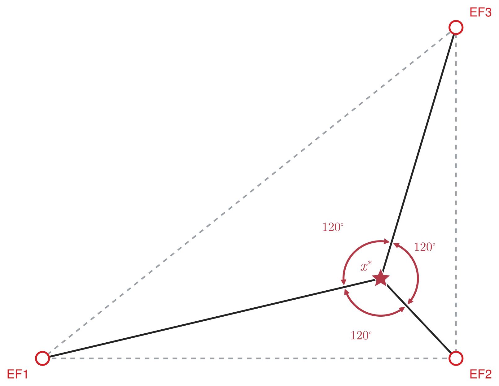
This problem was solved in 1629 by Fermat. For three points, the location that minimizes the total distance to them is a fourth point, the Steiner point, characterized by the three lines from it to the points meeting at equal angles of 120° (Fig. 9), the angle soap bubbles meet at as they settle into a natural minimum-energy state. Seen another way, if roads run from a first city to a second and from the second to a third, adding one intersection point and running three road segments to it covers less total distance than the two direct segments, which is why the major intersections of an interstate network typically sit at these minimizing points.
Figure 9: Fermat’s 1629 problem: for three points, the minisum location is the Steiner point, where the three lines to the points meet at 120°. Drawn for the three facilities of Ex. 2.
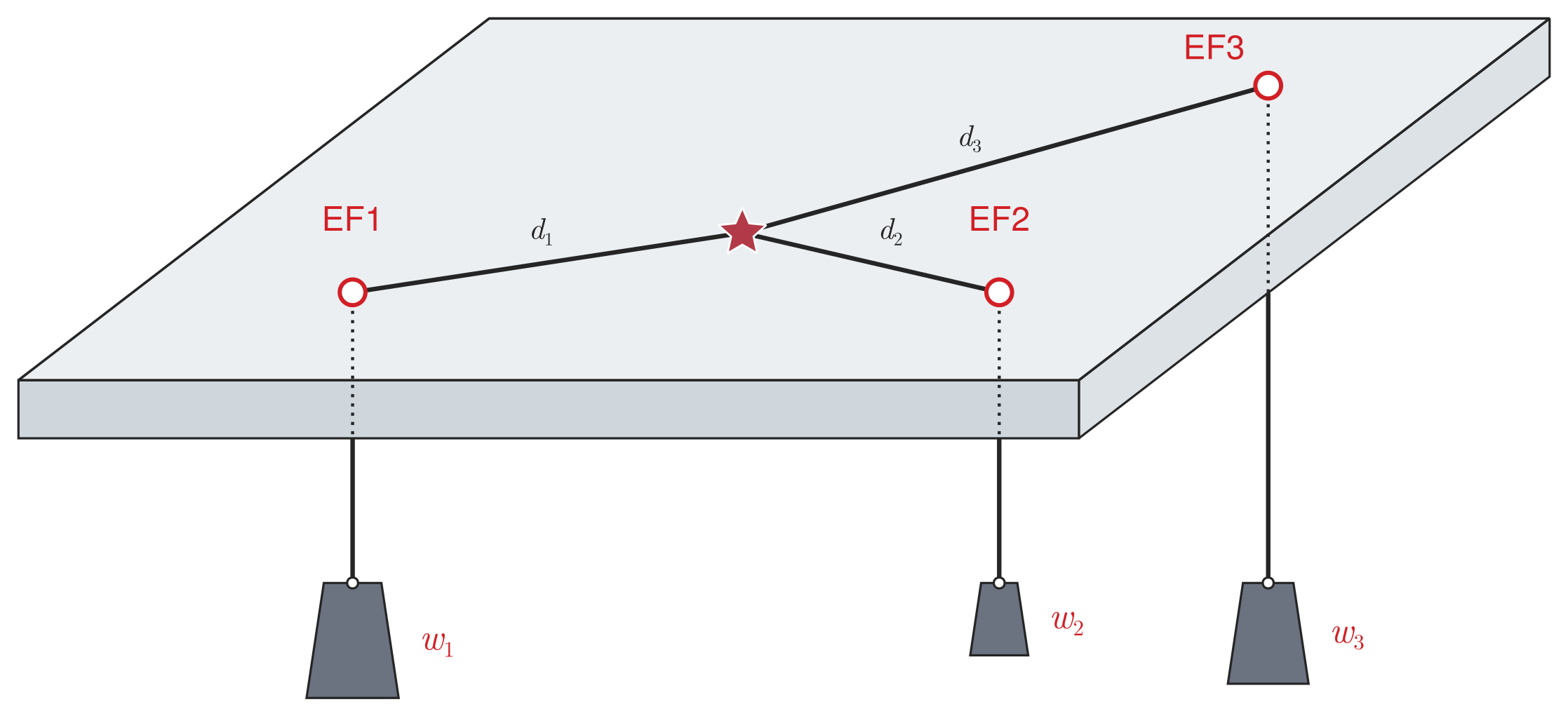
Before computers the weighted minimum was found mechanically, on what is called the Varignon frame (Fig. 10). Holes are drilled in a board at the existing facilities; a physical weight proportional to each facility’s monetary weight hangs from a string through its hole, the strings meet at a common ring, and the ring settles where it comes to rest, at the point that minimizes the total weighted distance. It is more accurate than the rectilinear approximation but far more work: photographs survive of two or three engineers in the 1930s spending three or four days on a single location this way, whereas the rectilinear-ordering shortcut of Lecture 2.1 is a twenty-minute exercise.
Figure 10: The Varignon frame: a string runs from a common ring through a hole at each existing facility, pulled by a weight proportional to that facility’s monetary weight w_i. The ring settles where it comes to rest, the weighted-minisum point.
The single-facility minisum is stated as a model carried from words to runnable code (Model 1). Its formulation is a math program in a generic distance; its implementation is a function given the weights, the facilities, and a distance function, returning the location, so the one model serves every metric the course uses.
The first is the location at which the total cost is smallest, and the second is that smallest cost, the objective evaluated at the optimum.
Reading \arg. The \arg operator extracts the argument corresponding to the operator it is applied to. \min_X TC(X) is the smallest cost; \arg\min_X
TC(X) is the X that produces it. The same holds for \arg\max. That is why the condition sits under \min: the minimization is what ranges over the candidate locations, and \arg is a separate operator applied to its result.
minimize: total weighted distance from the new facility to the m existing facilities
solve for:
(a) location X of the new facility, any point in the plane.
subject to: none
return: location X^\star of the new facility
assumptions:
(a) distance is a metric, for example the straight-line distance used below or the great-circle distance of Sec. 6;
(b) cost of each flow is proportional to distance, so each monetary weight w_i is a constant.
The implementation names no method. It builds the objective and hands it to Optim.optimize, the general-purpose optimizer of the Julia ecosystem, which searches numerically; how that search works, and why the result can be trusted, is taken up after the example. A numerical search of this kind must be given a point to start from, so minisum supplies one: x0, the centroid of the existing facilities. Whether that choice matters is taken up there too.
Not every minisum problem needs a search at all. If one existing facility carries at least half of the total weight, the optimum is at that facility, and no amount of searching will improve on it.
The condition is a majority in the literal sense, and the reason it determines the problem is that moving away from EF_j adds distance against more than half the weight while removing it from less than half. Lecture 2.3 returns to the theorem for several new facilities, where it determines which operations belong together rather than where a single facility goes.
When no facility holds a majority the location has to be found some other way. A Varignon frame does it mechanically: strings run from each existing facility over a pulley and carry a weight proportional to w_i, and the knot settles at the minisum point. The rest of this section does it numerically.
Example 2: Fermat’s 1629 problem
Determine the minisum location for three facilities of equal weight at (1, 1),(6, 1), and (6, 5), under straight-line distance.
Binding the data and a straight-line distance to Model 1 and calling its implementation gives the location directly.
# Code block 4: straight-line distance, the same as Logjam.d2d2(x1, x2) =length(x1) ==length(x2) ?sqrt(sum((x1 .- x2).^2)) :error("Inputs not same length.")P = [1.01.0; 6.01.0; 6.05.0] # three EFs, one per roww = [1.0, 1.0, 1.0] # equal weightsXᵒ =minisum(w, P, d2) # the minisum location
X^\star \approx (5.09,\ 1.97), the Steiner point of Fig. 9.
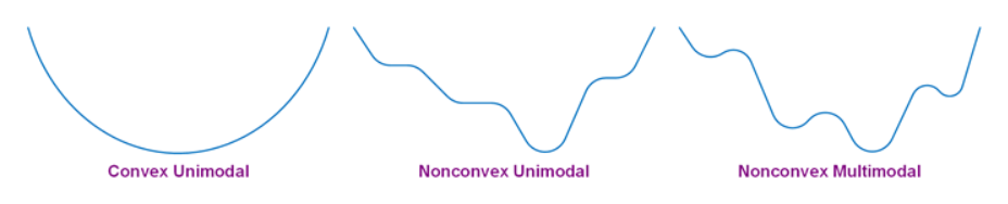
The search reached that point without any care about where it started, and the reason is the shape of the objective. When the objective is convex, a single bowl (Fig. 12), a downhill search reaches the bottom from wherever it starts, so any starting point gives the same optimum. The weighted-minisum objective is convex, so choosing a start is not a concern here. Nonconvexity by itself does not change that. An objective can be nonconvex and still unimodal, a single basin of irregular shape, and a downhill search reaches its one minimum from any start just as it does in the convex case. What makes the starting point matter is multimodality: several separate local minima, so that where the search begins determines which one it settles in (Fig. 11).
Figure 11: Convex unimodal, nonconvex unimodal, and nonconvex multimodal objectives. If convex or unimodal, any starting point will lead to the global optimum; otherwise, different starting points can lead to different local optima.
Show the code that generates this figure
# Code block 5: the total-cost surface over the planeusingCairoMakiexrng =0:0.1:7yrng =0:0.1:6Z = [sum(d2([x, y], P[i, :]) for i inaxes(P, 1)) for x in xrng, y in yrng]fig =Figure(size = (760, 320))a1, _ =contour(fig[1, 1], xrng, yrng, Z; levels =18, color =:steelblue4)scatter!(a1, P[:, 1], P[:, 2]; color =:firebrick)surface(fig[1, 2], xrng, yrng, Z; colormap =Reverse(:viridis), axis = (type= Axis3, azimuth =pi/4))fig
Figure 12: The objective for Ex. 2 is a convex bowl, drawn as contour lines (left, existing facilities in red) and as a surface (right). A single basin means a single minimum, reached from any start.
The optimizer steps downhill by one of two kinds of method. A gradient method, such as a quasi-Newton method, uses the objective’s derivatives; but since even simple location objectives rarely have an analytical gradient, it estimates one by finite differencing, which works well only on smooth objectives. A direct method, chiefly Nelder-Mead, never computes derivatives at all, reading only values of the objective, so it copes with the kinked or discontinuous objectives a gradient method cannot, less efficiently but far more robustly. Nelder-Mead is the basic method behind a spreadsheet’s Solver and the default in most optimization packages, and it is the default used here (Fig. 13).
Show the code that generates this figure
# Code block 6: the path Nelder-Mead takesTC(X) =sum(d2(X, P[i, :]) for i inaxes(P, 1))fargplot(f, x, kw) = (scatter!(x...; kw...); f(x))scatter(P[:, 1], P[:, 2]; color =:firebrick, markersize =11)kw = (; color = (:steelblue, 0.6), markersize =5)Xᵒ2=optimize(x ->fargplot(TC, x, kw), [0.0, 0.0]).minimizerscatter!([Xᵒ2[1]], [Xᵒ2[2]]; color =:red, marker =:star5, markersize =14)current_figure()
Figure 13: Nelder-Mead in action from (0,0): each blue dot is one evaluation of the objective; the search sweeps toward the optimum (red star), the existing facilities in firebrick.
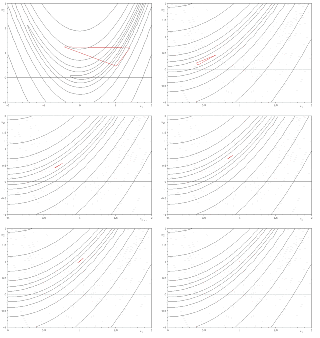
Nelder-Mead is also called the amoeba method, for the way it moves. It works a triangle of points across the plane, evaluating the objective at each: from the current triangle it tries a new point, and when that point improves on the worst corner it moves the triangle that way, creeping downhill by function evaluations alone. The step rules that determine each move are collected in the callout below; the working point is that the method needs nothing but the objective’s values (Fig. 14).
Figure 14: The simplex crawling downhill across a contour map: at each step it reflects its worst vertex through the opposite face, stretching when that helps and shrinking when it does not, until it closes on the minimum.2
NoteHow Nelder-Mead searches
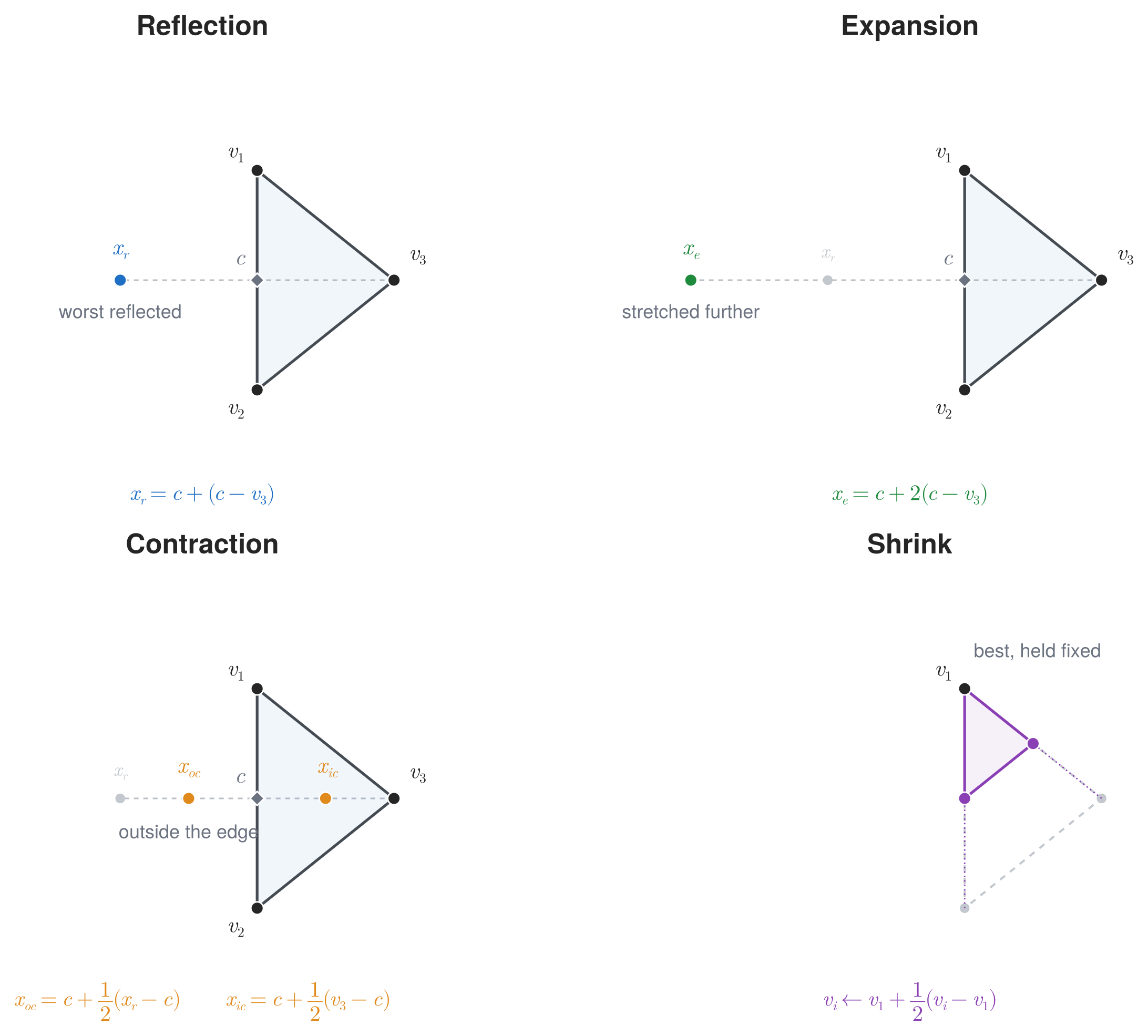
Each iteration orders the simplex’s corners from best to worst and tries to replace the worst. It first reflects that corner through the opposite edge: the reflected point is accepted if it is merely middling, stretched further by an expansion if it is the new best, and, if it is worse than the second-worst corner, pulled back by a contraction, taken outside the edge when the reflection still beats the current worst corner and inside when it does not. When even the contraction fails to improve, the whole simplex shrinks toward the best corner and the iteration restarts. The search reads only values of the objective, never its derivatives, which is what lets it handle kinked or discontinuous objectives a gradient method cannot.3Fig. 15 shows why the four moves are fewer decisions than they look: reflection, expansion and both contractions all step along the same ray through the worst corner and the centroid, differing only in how far, and shrink is the only one that leaves it.
Figure 15: The four moves on a two-dimensional simplex, with v_1 the best vertex and v_3 the worst. The centroid c of the remaining vertices sets the direction: reflection, expansion, and the two contractions all step along the same ray through v_3 and c, differing only in how far. Shrink is the exception, pulling every vertex halfway toward v_1 rather than replacing the worst.
algorithm nelder-mead;{ input: objective f; starting point x₀ ∈ ℝⁿ }{ output: a vertex minimizing f }begin form a simplex of n+1 vertices about x₀; repeat order so that f(v₁) ≤ f(v₂) ≤ ⋯ ≤ f(vₙ₊₁); c := centroid of the n best, v₁ … vₙ; { drop vₙ₊₁ } xᵣ := c + (c − vₙ₊₁); { reflection } if f(v₁) ≤ f(xᵣ) < f(vₙ) then vₙ₊₁ := xᵣ else if f(xᵣ) < f(v₁) then begin xₑ := c + 2(c − vₙ₊₁); { expansion } if f(xₑ) < f(xᵣ) then vₙ₊₁ := xₑ else vₙ₊₁ := xᵣ; end else if f(xᵣ) < f(vₙ₊₁) then begin x_c := c + ½(xᵣ − c); { outside contraction } if f(x_c) ≤ f(xᵣ) then vₙ₊₁ := x_c else shrink; end else begin x_c := c + ½(vₙ₊₁ − c); { inside contraction } if f(x_c) < f(vₙ₊₁) then vₙ₊₁ := x_c else shrink; end until the simplex is small enough; return v₁;end;{ shrink: replace each vᵢ, i = 2 … n+1, by v₁ + ½(vᵢ − v₁) }
4. Other types of location objectives
Lecture 2.1 set six objectives side by side in Table 1 in Lecture 2.1 without solving any. Three more of them can be solved here, on the same three facilities, by changing one line.
Minimax. The distances from the centroid to the three facilities are not equal, and the largest of them is what a minimax objective answers to.
# Code block 7: the centroid as a starting pointusingStatisticsx0 =mean.(eachcol(P)) # centroid startd2.([x0], eachrow(P))
The answer is nonsense, and loudly so: the facility has run off to 10^{154} and the objective to -\infty. Nothing was wrong with the code. On its own the maximin problem has no finite answer, since there is always somewhere further away.
A feasible region. Confining the facility to a rectangle makes the problem well posed. Outside the rectangle the objective is \infty, which the optimizer will not accept.
# Code block 12: a feasible region for the maximinr = [(0, 0), (7, 6)] # SW and NE corners of feasible regionisinrect(x, r) = r[1][1] <= x[1] <= r[2][1] && r[1][2] <= x[2] <= r[2][2]TC(x) =isinrect(x, r) ? -minimum(d2.([x], eachrow(P))) :InfTC([4, 4]), TC([8, 8])
Center of gravity. One more, and the gentlest: squaring each distance before summing gives the objective of Model 5 in Lecture 2.1. sum stays, and .^ 2 is the whole change.
# Code block 14: center of gravity, minimizing squared distanceTC(x) =sum(d2.([x], eachrow(P)) .^2)res =optimize(TC, x0)@show TCᵒ = res.minimumxᵒ = res.minimizer
The search returns its own starting point, because it began at the answer. Lecture 2.1 derived the closed form at Eq. 3 in Lecture 2.1: with equal weights the minimizer of squared distance is the plain centroid, which is exactly the x0 used throughout this section. Starting somewhere else and arriving at the same place is the check worth making.
optimize(TC, [0.0, 0.0]).minimizer # Code block 15: a different start
Figure 16: The same three existing facilities under four objectives. The bounded maximin sits on the edge of the region, which is what pins it; without the region it leaves the picture entirely.
Logjam does not have to implement all of these. Just using the Optim package alone does most of the work. Logjam just needs to supply any supporting infrastructure. In the case of maximin, it only becomes feasible when the region is bounded.
Optim and the plotting used here are general-purpose Julia. The logistics-specific layer that the rest of Location relies on, place names and distances over real geography, is introduced next.
5. Logjam: the logistics toolkit
The single-facility minisum of Sec. 3 was solved with optimize from Optim, a general-purpose optimizer taken from the Julia ecosystem. Logistics problems, though, are rarely posed in the language a solver expects: their data are place names, distances over real roads, and freight rates, not coordinate vectors and objective functions. Logjam is the Julia package written for this course to supply that missing layer. It does not reimplement what the ecosystem already does well, such as the optimization in Optim or the plotting in CairoMakie; it adds the logistics domain on top, turning place names into coordinates and measuring distance over real geography.
The distance and mapping functions the course needs were not available in any existing package, so they were gathered into a package of their own, Logjam. Packages in the general Julia registry are added by name; Logjam is still an early version and is not registered, so it is added instead by giving the URL of its GitHub repository, with registration by name left as a possibility for later.
Logjam collects tools across the logistics topics of the course: facility location, including discrete p-median and uncapacitated facility-location heuristics and continuous location by alternating location–allocation (ala) and the weighted center of gravity (wcentroid); transportation costing; network analysis and vehicle routing over the FAF5 highway network; a built-in U.S. gazetteer of cities, counties, and ZIP codes; forward and reverse geocoding; and the distance metrics used in this lecture.
The package cell in Lecture 1.2 adds Logjam by URL:
# Code block 17: adding Logjam by URLusingPkgPkg.add(url="https://github.com/mgkay/Logjam")
Its features activate through package extensions, so its capabilities grow as more packages are loaded: using Logjam alone provides the core location, costing, distance, and geocoding tools; adding CairoMakie enables plotting; adding GeoMakie as well enables the mapping functions, such as makemap and aligntext, used in Sec. 6. The facility-location and routing maps introduced in Lecture 1.1 were drawn with these same mapping tools, and the package’s README is the reference for its full function set. The remainder of this lecture puts Logjam to work computing the distances that the minisum objective needs.
6. Computing distances with Logjam
How can the distances between facility locations be determined? Since the transport is over the road, the natural answer is the road distance, but it is not computationally feasible to repeatedly calculate the actual road distances between locations. Each distance is a query against a road network: Google charges for access through its API and cuts a program off once it has used up its allowance, and the open-source alternative, OpenStreetMap, runs on servers that are limited.
The more basic obstacle is that most continuous locations examined during the Nelder-Mead procedure are not connected to a road. The procedure picks a point in two-dimensional space, and there is no reason that particular point will be on a road network, or even near one: it could be in the middle of a swamp.
The minisum objective needs a distance d(X, P_i) between the facility and each existing point. In the plane, that distance belongs to a family of metrics selected by a single parameter; over the curved surface of the earth, it is the great-circle distance. Logjam supplies both, together with the geocoding that turns place names into the coordinates they require. The planar metrics come first.
Given two points P_1 = (x_1, y_1) and P_2 = (x_2, y_2), a general metric distance function termed the l_p distance or norm can be used to represent several of the most common distances used in practice. The function uses different values of the parameter p to represent these special cases:
The above distances are defined for two-dimensional points, but they can be extended for points of any dimension. For 0 < p < 1, the l_p distance is not defined since the triangle inequality does not hold; for 1 < p < 2, the l_p distance lies between the rectilinear and the Euclidean distances; and for 2 < p < \infty, the l_p distance lies below the Euclidean distance and decreases as p increases.
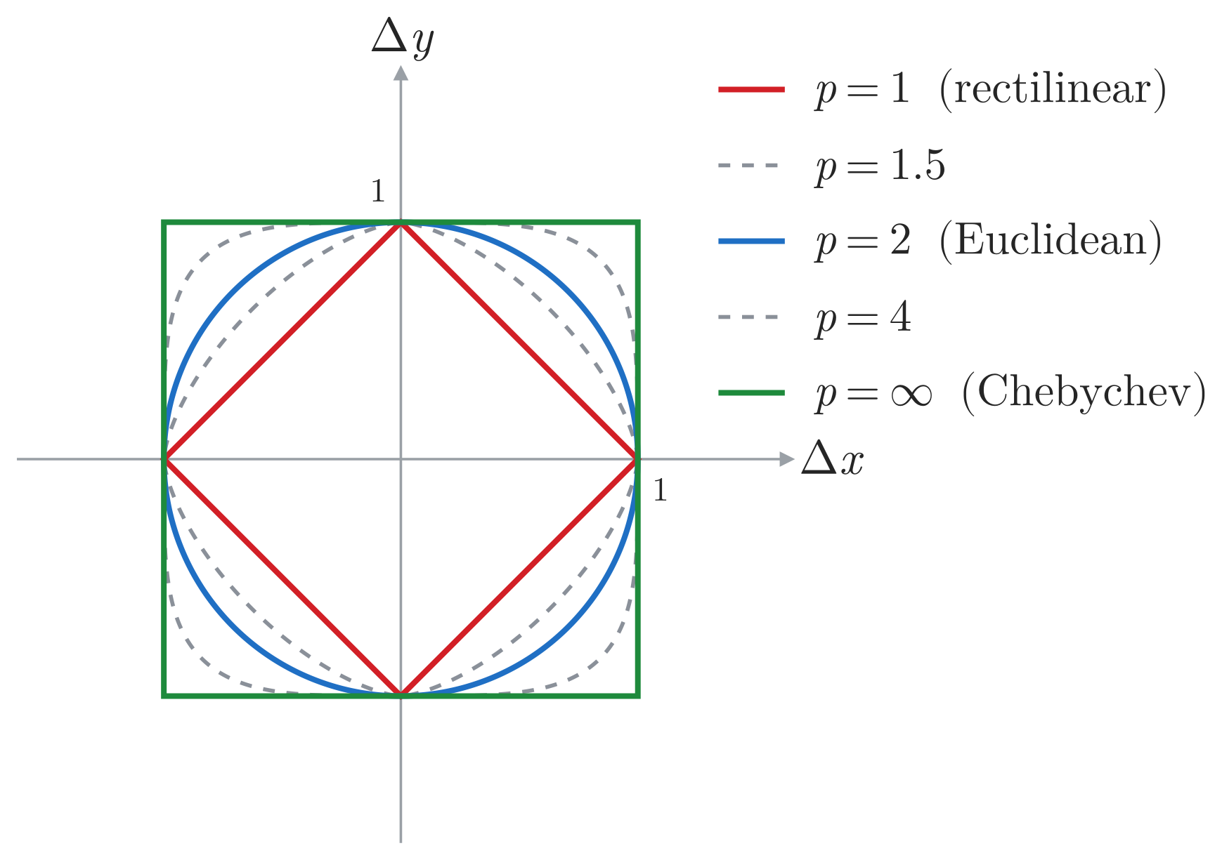
Each value of p has a characteristic contour of points at equal distance from the center (Fig. 17): a diamond for the rectilinear distance, the familiar circle for the Euclidean, and a square for the Chebychev, with the intermediate values filling the range between them.
Figure 17: Contours of equal l_p distance from the center for p = 1, 1.5, 2, 4, \infty: the rectilinear diamond, the Euclidean circle, and the Chebychev square.
Logjam computes each of these directly. d1 and d2 take two points; the unified dists takes point sets and a metric parameter, so a single call covers the whole family, down to the Chebychev limit at Inf.
# Code block 18: rectilinear and Euclidean distanceP1 = [0, 0] # two points in the planeP2 = [4, 3]d1(P1, P2), d2(P1, P2) # rectilinear, Euclidean
(7.0, 5.0)
# Code block 19: the l1, l2 and l-infinity metricsX1 = [00] # point sets, one row per pointX2 = [43][dists(X1, X2, p)[1] for p in (1, 2, Inf)] # l₁, l₂, l∞
3-element Vector{Float64}:
7.0
5.0
4.0
NoteProof of Chebychev distance
Without loss of generality, let P_1 = (x, y), for x, y \ge 0, and P_2 = (0, 0). Then d_\infty(P_1, P_2) = \max\{x, y\} and d_p(P_1, P_2) = (x^p + y^p)^{1/p}.
If x = y, then
\lim_{p \to \infty}(x^p + y^p)^{1/p}
= \lim_{p \to \infty}(2x^p)^{1/p}
= \lim_{p \to \infty} 2^{1/p}\, x = x .
If x < y, then
\lim_{p \to \infty}(x^p + y^p)^{1/p}
= \lim_{p \to \infty}\!\left[\left(\tfrac{x}{y}\right)^{p} + 1\right]^{1/p} y
= 1 \cdot y = y .
A similar argument can be made if x > y. ∎
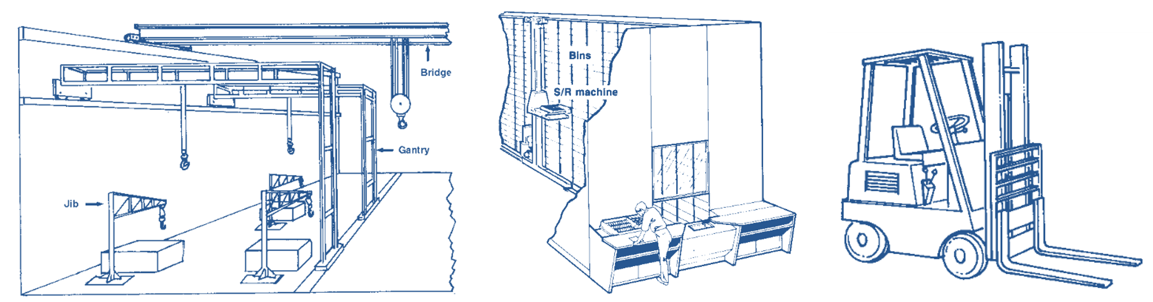
The Chebychev distance is the natural one when two motions run at once (Fig. 18), so travel time is set by the longer move: a lift truck drives down the aisle while raising its forks, and an overhead crane bridges and trolleys at the same time. A storage-and-retrieval machine in an automated warehouse is the third: it travels down an aisle of bins while its shuttle rises to the level of the bin, so the time from one bin to the next is the greater of the two motions. The book-retrieval system in the basement of Hunt Library works this way.
Figure 18: The three machines whose two motions run at once: overhead cranes, where the bridge travels while the hoist trolleys across it; a storage-and-retrieval machine serving an aisle of bins, where the carriage travels while the shuttle rises; and a lift truck, which drives and lifts together.4
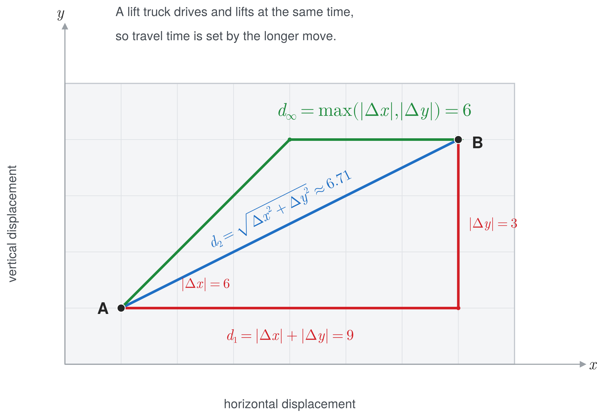
For a move with |\Delta x| = 6 and |\Delta y| = 3 (Fig. 19), the rectilinear distance adds the two (9) and the Euclidean takes the hypotenuse (\approx 6.71), but the time is set by the longer move alone, \max\{6, 3\} = 6.
Figure 19: One move from A to B under the three metrics: rectilinear d_1 = 9, Euclidean d_2 \approx 6.71, and Chebychev d_\infty = \max\{6, 3\} = 6, the longer of the two displacements.
The great circle distance is an exercise in spherical trigonometry. A compact formula gives the separation of two points as an angle in radians, as though on a sphere of unit radius; that angle becomes a distance by multiplying it by the radius of the earth.
Great circle, or geodesic, distances on the surface of a sphere, such as the earth, are the shortest distance between two points on the surface along the circle formed by the intersection of the surface and a plane passing through the center of the sphere (a “great circle”). The elevations of the points on the surface are usually ignored.
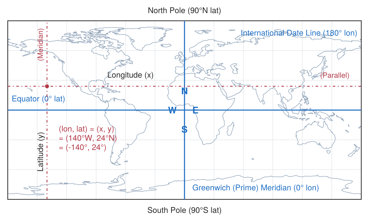
A point on the surface of the earth is located by its longitude and latitude (Fig. 20). Longitude is measured east and west of the Greenwich prime meridian, latitude north and south of the equator. East and north are positive and west and south are negative, so a point at 140°W, 24°N has coordinates (lon, lat) = (x, y) = (-140°, 24°).
Figure 20: Longitude and latitude for points on the surface of the earth. Longitude runs from the Greenwich prime meridian (0° lon) to the international dateline (180° lon), and latitude from the equator (0° lat) to the poles (90°N and 90°S lat).
The great circle distance d_{GC} between points 1 and 2 on the surface of the earth, specified by their longitude (lon) and latitude (lat) angles in radians, is d_{GC} = R\,d_{rad}, where R is the radius of the earth and the central angle d_{rad} (in radians) is
Coordinates are often published in degrees, minutes, and seconds rather than in decimal degrees. To convert degrees (DD:MM:SS) to decimal degrees, with the hemisphere setting the sign:
x_{deg} = \begin{cases}
DD + \dfrac{MM}{60} + \dfrac{SS}{3{,}600}, & \text{if E or N}\\[2ex]
-DD - \dfrac{MM}{60} - \dfrac{SS}{3{,}600}, & \text{if W or S}
\end{cases}
\tag{12}
Raleigh, at 78°39′32″W and 35°49′19″N, is (-78.659, 35.8219) in decimal degrees, the pair used below.
NoteDerivation of the great circle distance
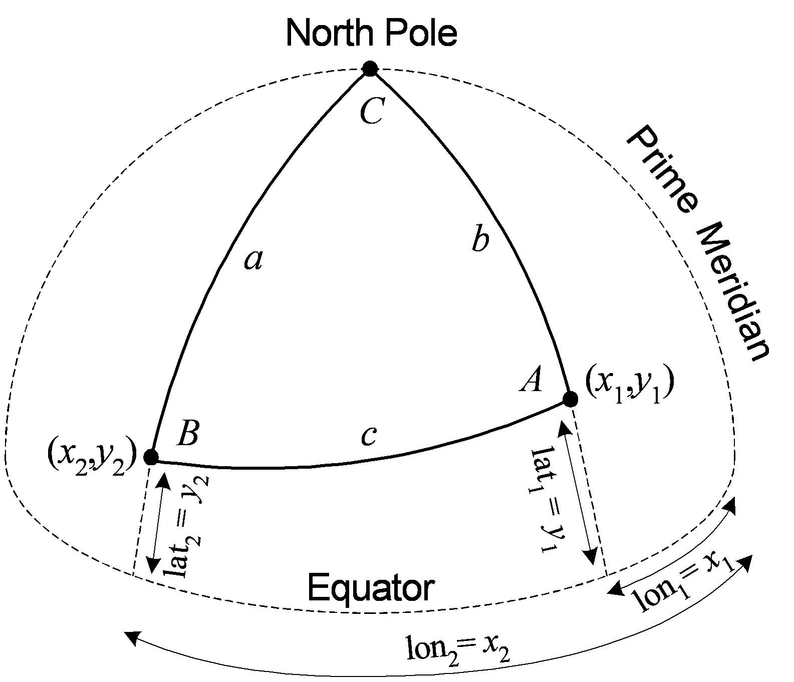
In Fig. 21, a,b, and c are the sides of a spherical triangle and A,B, and C are the corresponding angles. The great circle distance between points 1 and 2 in radians (d_{rad}) corresponds to side c of the triangle.
Figure 21: Great circle distance derivation.
Given
a = 90^\circ - y_2, \quad b = 90^\circ - y_1, \quad C = x_1 - x_2
the formula for great circle distances can be derived using the spherical law of cosines for sides:
d_{rad} = c = \cos^{-1}\!\left[\sin(y_2)\sin(y_1)
+ \cos(y_2)\cos(y_1)\cos(x_1 - x_2)\right]
The above formula can result in round off error if the two points are located at exactly opposite sides of a sphere. Instead, the Haversine formula can be used (Eq. 10). The Haversine formula does not need to be used if the great circle distance is being calculated by hand and the two points are known to not be on opposite sides of the sphere.
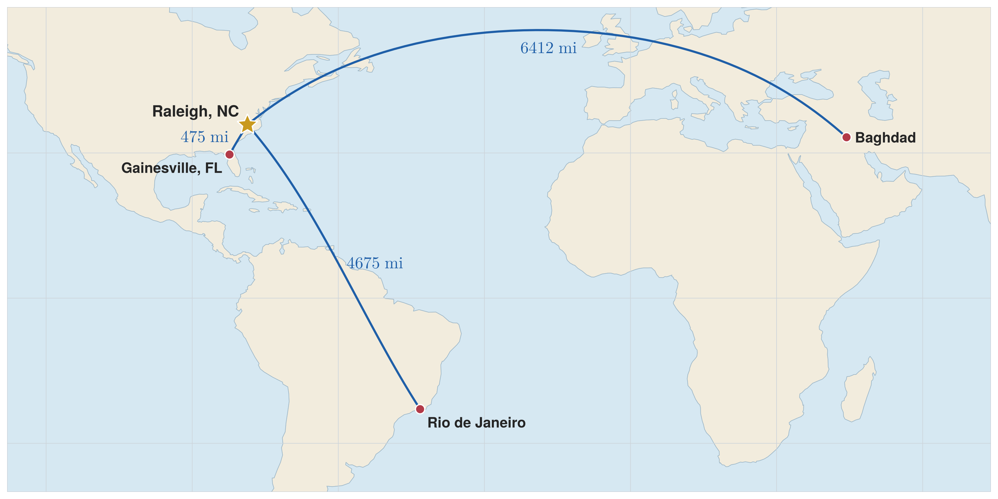
The formula applied to a few points shows how far apart the distances can be. A worked example measures three cities from Raleigh, each given as a (longitude, latitude) pair in decimal degrees; dists with the :mi unit (or :rad) returns the great-circle distance to each. Fig. 22 draws the same three distances on the globe. Each arc is the shortest path there is between its two points, and none of them is the straight line a flat map would draw between the same pair.
# Code block 20: great-circle distance to three citiesRaleigh = [-78.65935.8219] # one point, as a rowXY = [-82.33629.6742# Gainesville, FL44.366733.2333# Baghdad-43.2-22.95] # Rio de Janeiroprt(DataFrame( City = ["Gainesville, FL", "Baghdad", "Rio de Janeiro"], Radians =vec(dists(Raleigh, XY, :rad)), Miles =vec(dists(Raleigh, XY, :mi))))
City Radians Miles
────────────────────────────────────
Gainesville, FL 0.12 475.37
Baghdad 1.62 6,412.00
Rio de Janeiro 1.18 4,675.44
Figure 22: Great-circle distances from Raleigh, drawn as arcs on the globe: 475 miles to Gainesville, 4675 miles to Rio de Janeiro, and 6412 miles to Baghdad, the values computed above.
A great-circle distance needs coordinates, and Logjam carries a built-in gazetteer of U.S. places to supply them. usplace() returns every city, town, and census-designated place as a table of names, coordinates, and populations; filter with st2fips, the state’s numeric code, narrows it to the places of interest, here the ten North Carolina cities above one hundred thousand people.
# Code block 21: NC cities over 100k, from the Logjam gazetteerdf =filter(r -> r.STFIP ==st2fips(:NC) && r.POP >100_000, usplace())select!(df, :NAME, :LON, :LAT, :POP)prt(df)
NAME LON LAT POP
───────────────────────────────────────
Cary -78.82 35.78 174,721
Charlotte -80.83 35.21 874,579
Concord -80.64 35.39 105,240
Durham -78.90 35.98 283,506
Fayetteville -78.97 35.08 208,501
Greensboro -79.83 36.10 299,035
High Point -79.99 35.99 114,059
Raleigh -78.64 35.83 467,665
Wilmington -77.89 34.21 115,451
Winston-Salem -80.26 36.10 249,545
Each row’s longitude and latitude are one point P_i, and dgc returns the great-circle distance between two of them. Raleigh to Charlotte is about one hundred thirty miles, as the crow flies.
# Code block 22: Raleigh to Charlottell(nm) =collect(filter(r -> r.NAME == nm, df)[1, [:LON, :LAT]])xyR =ll("Raleigh") # (lon, lat) in degreesdgc(xyR, ll("Charlotte")) # great-circle miles
130.3903764072013
Broadcasting dgc over the whole set gives Raleigh’s distance to every city at once, and the standard index queries answer the natural questions: the farthest city, and the three nearest.
# Code block 23: the farthest city from Raleighpt =collect.(zip(df.LON, df.LAT)) # one [lon,lat] per cityd =dgc.([xyR], pt) # Raleigh to each citydf[argmax(d), :NAME] # farthest city
"Charlotte"
df[sortperm(d)[2:4], :NAME] # Code block 24: three nearest, skip Raleigh
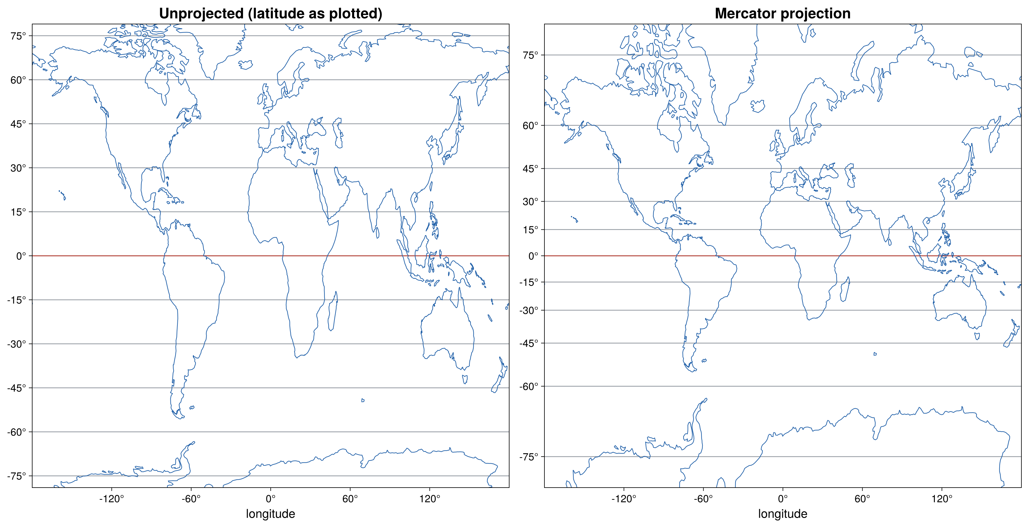
Plotting longitude and latitude directly on flat axes distorts the map, so the geography is shown through a projection. The most convenient here is the Mercator projection, which has the useful property that a straight line between two points is a constant compass bearing, the line a navigator would steer.
The projection leaves longitude unchanged and stretches the latitude axis toward the poles, placing a point at latitude \varphi at ordinate \sinh^{-1}(\tan\varphi), so equal steps of latitude spread apart with distance from the equator. Writing that ordinate y_{proj}, the transform inverts as \varphi = \tan^{-1}(\sinh y_{proj}), which recovers a latitude from a projected ordinate. Logjam’s makemap applies the projection through GeoMakie, so the maps in this section are already Mercator-projected; Fig. 23 shows the effect on a world coastline.
Figure 23: The same world coastline drawn with latitude plotted directly (left) and under the Mercator projection (right). Both carry the same latitude labels, but on the right they sit at their projected positions, so equal steps of latitude spread apart toward the poles.
These distances feed straight back into the single-facility minisum. The model of Model 1 never depended on the metric, so the same objective, now with the great-circle distance in place of the straight-line one, locates a facility over real geography. Taking each place’s population as its weight w_i turns the objective into total population-weighted travel, and its minimizer into the location that is, on average, closest to everyone.
Example 3: NC Zoo
Locate a single facility to minimize the total population-weighted great-circle distance to every place in North Carolina.
Every place enters, not just the large cities: usplace filtered to the state, each place weighted by its population, with the weighted centroid wcentroid as the starting point for the search.
The nearest place names the answer. Fig. 24 sets that optimum against every place in the state, which is what makes the result readable: the ten largest cities are labeled, and the population-weighted optimum sits near none of them.
# Code block 26: the place nearest that optimumd =dgc.([xyᵒ], pt) # optimum to each placedf[argmin(d), :NAME], round(minimum(d)) # nearest place, miles
("Franklinville", 6.0)
The optimum lies about 6 miles from Franklinville, near the geographic center of the state.
Show the code that generates this figure
# Code block 27: the optimum drawn against the ten largest citiesusingGeoMakiebig =sort(filter(r -> r.POP >100_000, df), :POP, rev =true)nbig =nrow(big)zoo = [-79.7645, 35.6295] # NC Zoo, near Asheboroefc = colorant"#d21f26"# the citiesoptc = colorant"#b23a48"# the optimumzooc = colorant"#1e8a3c"# the zooink = colorant"#252525"fig, ax =makemap(big.LON, big.LAT)scatter!(ax, big.LON, big.LAT; markersize =11, color = efc)# labels auto-place, except Charlotte: its dot sits on the borderich =findfirst(==("Charlotte"), big.NAME)oth =setdiff(1:nbig, ich)text!(ax, big.LON[oth], big.LAT[oth]; text = big.NAME[oth], color = ink, fontsize =18,aligntext(big.LON, big.LAT; offsetamt =1, idx = oth)...)text!(ax, [big.LON[ich]], [big.LAT[ich]]; text = ["Charlotte"], color = ink, fontsize =18, align = (:right, :center), offset = (-12, 4))scatter!(ax, [xyᵒ[1]], [xyᵒ[2]]; marker =:star5, markersize =20, color = optc)text!(ax, xyᵒ[1], xyᵒ[2]; text = L"x^*", color = optc, fontsize =20, align = (:left, :bottom), offset = (10, 6))scatter!(ax, [zoo[1]], [zoo[2]]; marker =:diamond, markersize =13, color = zooc)text!(ax, zoo[1], zoo[2]; text ="🦒 NC Zoo", color = zooc, fontsize =18, align = (:left, :top), offset = (8, -6), font ="Segoe UI Emoji")fig
Figure 24: The population-weighted minisum over every place in North Carolina (the ten largest cities labeled). The optimum x^* (star) sits in the central Piedmont, within a few miles of the North Carolina Zoo near Asheboro.
The proximity of the population-weighted minisum location to the location chosen for the North Carolina Zoo near Asheboro seems most likely to just be coincidental. The minisum location is the one that, on average, minimizes the distance everyone in the state must travel, which would be a natural criterion for a facility the whole public visits. A zoo is such a facility. Accounts of the site’s selection do mention its central position in the state, but none gives evidence that centrality was a principal factor in the decision.5 Given what computing could routinely support in the early 1970s, it is also unlikely that a decision of that period rested on an analysis of the kind carried out here.
7. Circuity factors
The great-circle distance was used in Ex. 3 to determine the location that minimized the total population-weighted distance from all of the places in North Carolina. The total person-miles corresponding to the optimal location actually understates the total miles people would travel to this location: the great-circle distance was used, and real people travel on actual roads, so they cover slightly longer distances than that. With respect to determining the location, using the actual road distances traveled by people from all of the thousands of places in North Carolina would not significantly change the location found. The only time knowing the actual road distance is helpful in a location problem like this is when there is some cost associated with the distances actually traveled; for example, if people actually paid by the mile to reach the location. Since it would be quite time-consuming to determine thousands of actual road distances, a convenient approximation to them can be obtained using the circuity factor.
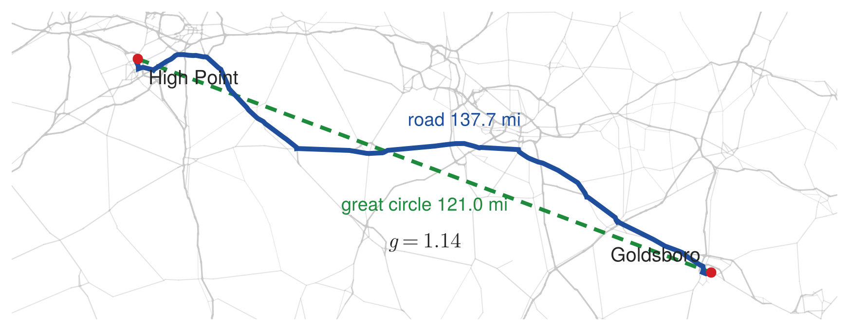
A straight line between two points is not a distance anyone travels. The great-circle distance from Goldsboro to High Point, North Carolina is 121 miles; the shortest-travel-time road route between them, traced through the road network in Fig. 25, is 137.7 miles. The ratio of the two is the circuity factor,
g = \frac{\text{road distance}}{\text{great-circle distance}},
\tag{13}
which for this pair is 137.7/121.0 = 1.14.
Figure 25: Road route against great-circle distance, Goldsboro to High Point, North Carolina. The dashed line is the great circle; the solid line is the shortest-travel-time path through the road network.
A single origin-destination pair gives a single ratio, which on its own is not useful. What makes the factor useful is a small sample. Great-circle distance is cheap to compute for any pair of coordinates, and the corresponding road distance can be read off a mapping service. Such a service usually returns several routes rather than one, and the right choice is the shortest travel time, which may be slightly longer in miles, because that is the route a truck would actually take.
Given n sampled pairs, the factor is the average of their ratios,
g = \frac{1}{n}\sum_{i=1}^{n} \frac{d_{road_i}}{d_{GC_i}},
\tag{14}
and it is then applied the other way round, to estimate a road distance that was never looked up:
d_{road} \approx g \cdot d_{GC}(P_1, P_2).
\tag{15}
Estimating a circuity factor
The circuity factor depends on both the trip density and the directness of the travel network. A good default value for road travel is 1.2. The factor in high-density areas is usually lower, because there are more direct roads between two large cities. Circuity factors for rail travel are higher than for road travel, because the rail network is far less dense. In sparse country, where the roads are few, they also run less directly, so the factor there is higher than in a dense region.
Just 5 to 10 sampled road pairs give a reasonable estimate, as long as the samples are independent and do not overlap, because the overestimates tend to cancel the underestimates. The sample can be smaller than that rule of thumb suggests, since three pairs are already serviceable. Where a factor is to be used extensively, the samples can be weighted toward the higher trip densities, but in practice that refinement is rarely needed.
The procedure is short enough to run in full. Take the three cities of Fig. 26, sample the three pairs among them, and average the ratios. The great-circle distances are computed; the road distances are looked up once and taken as data, which is what a handful of samples means in practice.
The three factors differ, and averaging them is the whole method: the pair that overstates the region is offset by the pair that understates it.
\bar g = 1.13
An average of three ratios is a claim, and it can be checked. The pair this section opened with, Goldsboro to High Point, took no part in the calibration: different state, shorter trip, and a road distance measured over the network rather than looked up. Applying the estimate to it and comparing against what that pair actually gives is the test.
# Code block 30: the estimate against a held-out pairgGH =137.7/121.0# road / great-circle, held out(held_out =round(gGH, digits =3), estimate =round(ḡ, digits =3), error_pct =round(100* (gGH - ḡ) / gGH, digits =1))
Under one percent, from three samples in another part of the country. That is what “three pairs are already serviceable” means, and it is worth doing rather than assuming: a held-out pair is the only thing that distinguishes a factor that generalizes from three ratios that happen to average out.
An estimated factor is the wrong tool in three cases, and the actual road network should be used instead:
Few distances are needed, in which case a mapping service answers directly.
Distances are short, since short trips have fewer direct roads available and so scatter more widely around any average.
Obstacles, such as water or mountains, limit direct road travel and make the local factor unlike the regional one.
Across most of the eastern United States the factor stays in the neighborhood of 1.15 to 1.25, which is why 1.2 serves as a default at all.
In general, estimated circuity factors can vary quite extensively depending on the particular road network, with typical values ranging from 1.05 all the way to 1.35. This matters in particular later, when actual road networks are being used. It is often necessary to connect an isolated location to the road network because small residential connector roads may not be part of the road network. In such cases, what is being estimated is a short distance, and there may not be an actual road that is convenient. Since the distance is short, the value is not going to impact things too much, so a reasonable estimate to use can be as high as 1.4 to 1.5.
What circuity changes, and what it does not
A circuity factor multiplies every distance by the same constant. That single observation determines how it enters a location decision, and the answer has two halves that are easy to run together and should not be.
A circuity factor does not change the optimal location, because scaling every distance by a constant leaves the minimizing point unchanged. It does change total cost, because the transport rate r is in dollars per ton-mile, so the miles it multiplies must be the miles actually driven.
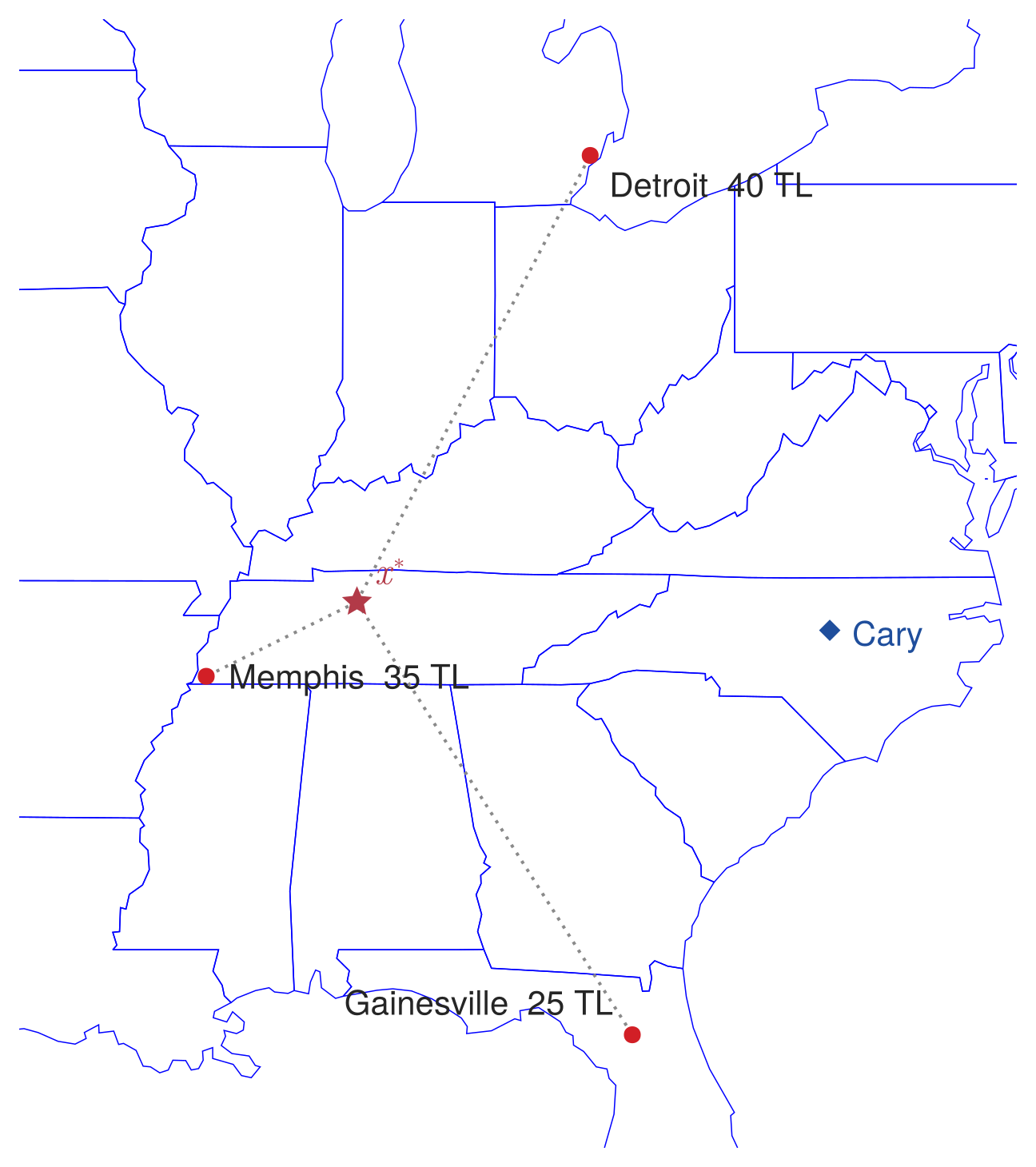
The consequence is that circuity matters exactly where cost, not position, is the question being asked, and the most common such question is what an alternative site would cost. Fig. 26 is that comparison: the optimum falls inside the triangle of the three existing facilities, and Cary, the site the firm would prefer on other grounds, falls outside it.
Figure 26: Locating for existing facilities at Detroit, Gainesville and Memphis, with Cary as the alternative site. The optimum falls inside the triangle formed by the three cities; Cary lies outside it.
Example 4: Price of staying in Cary
Determine the new-facility location serving existing facilities at Detroit, Gainesville and Memphis, receiving 40, 25 and 35 truckloads per year, and determine the increase in annual transport cost at $2.00 per loaded mile if the facility is instead placed at Cary, North Carolina.
The framing is a consulting one. A company whose owners are already in Cary would prefer to stay there, everything else being equal. Transport cost is not the whole of their decision: for a distribution company it is close to everything, but for a company that has to hire engineers and technical staff it might be half, with the rest going to who is willing to live in the location, the cost of energy, tax policy, and a long list besides. So the question put to the logistics engineer is not where to locate. It is what staying in Cary costs per year against the transport-optimal site. If the answer is a few hundred dollars a month the company stays; if it is millions, it moves. Producing that differential is the whole of the engineer’s task, and the trade against wages, taxes and energy is management’s.
In order to determine the differential, the transport rate is needed and is the piece of information a firm usually does have: say $2 per mile for a truck on the road. Evaluated against great-circle distance, the resulting estimate of transport cost is too low, because those are not the miles the truck drives. Where that rate comes from is taken up in Transport.
The three customers are the cities sampled for circuity in code block 28, each defined there as a [longitude, latitude] pair in degrees. Those cities and their truckloads are the data; the factor \bar g just estimated turns great-circle miles into road miles, and the rate turns road miles into dollars.
# Code block 31: truckload weights and the annual costP =permutedims(hcat(Detroit, Gainesville, Memphis)) # lon/lat, blk 28wTL = [40.0, 25.0, 35.0] # truckloads per yearrate =2.00# $ per loaded mileTCyr(xy) = rate * ḡ *sum(wTL[i] *dgc(xy, P[i, :]) for i in1:3)
TCyr (generic function with 1 method)
The optimum is found the way 2.2 found one, a downhill search from the weighted centroid.
# Code block 33: what an alternative site would costCary = [-78.8190, 35.7814]Δ =TCyr(Cary) -TCyr(xᵒ)prt(DataFrame( Site = ["optimum", "Cary, NC", "increase"], Cost =round.([TCyr(xᵒ), TCyr(Cary), Δ], digits =0)))
Site Cost
───────────────────
optimum 87,149
Cary, NC 122,536
increase 35,386
Staying in Cary costs about $35.4k per year more than the transport optimum, an increase of 40.6%.
That is the number the engineer hands over. Whether it is worth paying is not a transport question.
→ Circuity is the correction that turns a geometric answer into a monetary one. The location survives the correction; the number attached to it does not.
8. FedEx hub choice
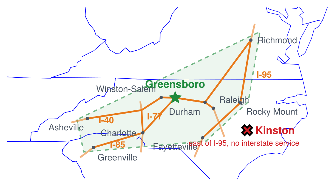
The population-weighted minisum location is a continuous answer, free to fall anywhere. A real single-facility decision usually chooses among a handful of actual sites, and one such choice played out in North Carolina. When FedEx was siting its Mid-Atlantic ground hub, the state weighed offering incentives to draw it to the North Carolina Global TransPark at Kinston, in the east. Kinston is a weak ground-hub site: it lies east of I-95, the easternmost interstate, and is served by no interstate of its own. Greensboro, by contrast, sits at the crossing of I-40 and I-85, central to Charlotte, the Triangle, and the Triad (Fig. 27).
An analysis carried out for the state, without access to FedEx’s own figures, used the guesstimation methods of Lecture 1.1 to put the annual cost penalty of the Kinston site over Greensboro at roughly $12 million a year, the size of the subsidy it would take to offset it. Years later a FedEx analyst who had run the company’s own internal study put the figure within a million or two of that estimate, a striking check on guesstimation for a quantity no outsider could measure directly. FedEx built its hub at Piedmont Triad International in Greensboro; the TransPark, long criticized for its distance from major highways, did not win it.6
Figure 27: FedEx hub choice: Greensboro (star) at the I-40/I-85 crossroads versus Kinston (✕), east of I-95 with no interstate service.
The population-weighted center and the FedEx decision point the same way, to the central Piedmont, and together they close the loop opened in Lecture 2.1: where a facility sits is a long-lived, costly commitment, and the tools of this lecture, distances over real geography and a minisum solved numerically, are what turn that commitment into a computation. Choosing among discrete candidate sites, rather than a free point in the plane, is the subject the next lectures take up.
J. C. Lagarias, J. A. Reeds, M. H. Wright, and P. E. Wright, “Convergence Properties of the Nelder-Mead Simplex Method in Low Dimensions,” SIAM Journal on Optimization 9, no. 1 (1998): 112–147.↩︎
Cranes, Fig. 103 in Reference Guide to Overhead Material Handling Systems, Charlotte, NC: Material Handling Institute, 1993. Storage-and-retrieval machine, Fig. 6-14, and lift truck, Fig. 7-7, both in R.A. Kulwiec, Advanced Material Handling, Pittsburgh, PA: Material Handling Institute, 1983.↩︎
The zoo’s site was chosen in 1971 from six candidates, Albemarle, Concord, Statesville, Butner, Chatham County, and Asheboro, after a two-year search by a state site-selection committee; the conditions set for it were a parcel of at least 1,000 acres and a pledge of at least $150,000 from the host community. “The 1970s: Room to Roam at the North Carolina Zoo,” Our State, https://www.ourstate.com/the-1970s-room-to-roam-at-the-north-carolina-zoo/ (accessed August 2026). The chosen parcel, near Purgatory Mountain in the Uwharrie range of Randolph County, is described as lying “near the geographic center of the state”: William S. Powell, “North Carolina Zoological Park,” NCpedia, 2006, https://www.ncpedia.org/north-carolina-zoological-park (accessed August 2026). Neither account gives distance to the state’s population as a selection criterion, and the center computed in this example is population-weighted rather than geographic.↩︎
FedEx sited its Mid-Atlantic hub at Piedmont Triad International Airport in Greensboro; the North Carolina Global TransPark at Kinston was the promoted alternative, frequently criticized for its location away from major highways. “Global TransPark Seeks FedEx Hub,” WFMY News 2 (2003), https://www.wfmynews2.com/article/news/local/global-transpark-seeks-fedex-hub/83-404033858.↩︎