
1.3: System Performance Estimation
ISE 754: Logistics Engineering, Fall 2026
The value of approximate analytic solution remains, because it often gives a deeper understanding which complements and illuminates the results of numerical computation.
— J. F. C. Kingman1
Lecture 1.1 built models with a small vocabulary that separated two things a model does: describe a system, or prescribe a change to it. Used descriptively, a model predicts how a given solution will perform; used prescriptively, it searches across solutions for a good one. This lecture is the descriptive side, performance estimation: given a system, real or proposed, predict how it will operate. The prescriptive side, optimization, comes later, and depends on this one, no search over designs is possible until a design can be evaluated.
Lecture 1.1 also estimated parameters at different levels of effort: level 0, guesstimation, brackets an unknown with a quick low and high; level 1, mean-value analysis, works with averages; level 2, nonlinear models, brings in variability and more structure. Performance estimation uses the same levels, but what it estimates is now a measure of how the whole system operates: its cost, its profitability, its throughput, its cycle time, the work waiting in it, or whatever the decision at hand turns on. Any level can produce such an estimate; the level sets only how faithfully the model represents the system, and so how accurate the estimate is. A guesstimate or a linear, average-based model is often enough. But some systems are governed by their bottlenecks and their variability rather than their averages. Queues form from variation even when average capacity looks ample, and a line is paced by its tightest constraint. There, a level-2 model, nonlinear and variability-aware, represents the system far better. The cycle-time estimate developed later in this lecture is one such model. One level higher, level 3, simulation, also makes its first appearance in this lecture (Sec. 7): where interactions grow too complex for any formula, the system is played out event by event instead.
Two approaches run through the lecture. When a system resists a direct model, its performance can be bracketed between an easy best case and an easy worst case. When its load and variability can be modeled, a direct model estimates the performance outright. The bracket is the failsafe; the direct model is the sharper estimate when it applies.
1. Bracketing
Bracketing is the first and most general way to estimate a system’s performance, and it needs no detailed model. For many systems that resist a direct model, two extreme cases are each easy to model. Perfect control, the most orderly the system could run, has no variability and gives the best-case (lower) bound. No control, fully random behavior, is the “totally random” case (a Poisson process, Sec. 4) and gives a practical worst-case (upper) bound. A single estimate then follows from the geometric mean of the two, the same lower-bound/upper-bound move used for a single parameter in Guesstimation (Ex. 1 in Lecture 1.1), now applied to whole-system performance. A real system sits between the extremes, and the geometric mean places the estimate there. (Genuinely bad control, which actively bunches or batches work, can be worse even than no control, so “no control” is a practical upper bound, not an absolute one.) This is a general-purpose failsafe; it has rescued many systems that would otherwise be almost impossible to model.
The waiting time for a bus is the canonical instance. The headway is the time between consecutive buses. Under perfect control the buses run on an evenly spaced schedule, so a passenger arriving at a random moment waits, on average, half the headway. Under no control the buses arrive at random (a Poisson process, Sec. 4), and the average wait is the full headway, not half. The reason is the memorylessness of random arrivals: however long the wait has already lasted, the expected time to the next bus is still a full average headway; equivalently, a passenger is more likely to arrive during a long gap than a short one, so the long gaps dominate the average wait.
Example 1: Bus waiting time
Estimate the waiting time for a bus when the headway (the average time between buses) is 8 minutes and passengers arrive at random, with no real-time bus tracking.
With headway h = 8 min, perfect control gives a wait of h/2 (lower bound) and no control gives h (upper bound). The geometric-mean estimate is
\text{wait} = \sqrt{\tfrac{h}{2}\cdot h} = \sqrt{\tfrac{8}{2}\cdot 8} = \sqrt{32} \approx 5.66\ \text{min}.
Estimated waiting time ≈ 5.66 min
Perfect control is not merely hypothetical. A campus trolley system developed by John Bartholdi and used at Georgia Tech instructs each bus how long to hold at a stop, so that it does not close the gap on the bus ahead, and the fleet stays evenly spaced. Left uncontrolled, buses bunch: one fills while the one behind it runs nearly empty, and capacity goes unused.2
2. Production systems
Another way of viewing logistics engineering is that it involves the design and operation of a logistics system, which is itself a type of production system. From this perspective, manufacturing, service, and logistics systems are all different types of production systems:
- Manufacturing systems: produce a good; can own/control (inanimate) thing → inventory possible; provide form utility.
- Service systems: produce a service; do not own the person or thing → inventory not possible; provide general work utility.
- Logistics systems: provide time/place utility; support manufacturing and service systems.
Given the design of a good/service and process, production system design involves determining the production capacity and logistics needed to actually provide the good or service. What makes production-system design hard:
- Things not always where you want them, when you want them.
- Resources are lumpy.
- Things vary.
Transport and location methods, the focus of logistics, are used to answer the where, while inventory methods are used to answer the when. Lumpy resources imply that there is a minimum effective size for most resources, below which it is too costly to operate. These lumpy resources typically involve some type of fixed cost that is independent of the scale of operation, which lead to economies of scale and scope. The same lumpiness applies to skill: a resource must be skilled enough for the hardest task it may face, which sets a floor on the scale that can use it fully. A highly trained specialist cannot be kept on call at every small clinic for a case that arises once a month; remote delivery is one way to bring that capability to a smaller scale.
The fact that both demand for the output of a production system, along with the production process itself, can vary is the major source of operating problems. Variability can be known or unknown. Unknown variability is referred to as uncertainty or randomness, which can be dealt with by various types of buffering. Known variability includes things like variations in seasonal demand that are predictable and as a result can often be more effectively handled by building inventory, for example, during periods of low demand. Also, bad control of a production system can lead to high variability.
Variability is absorbed by one of three buffers, and only three:
- capacity: machines or servers held in reserve;
- time: customers made to wait, or demand spread out through reservations and appointments;
- inventory: stock built ahead of need.
Known variability, such as a season that concentrates most of a year’s demand into two months, admits two strategies: produce at a level rate all year and hold the surplus as inventory, or idle the plant and ramp up just before the season. Obsolescence determines the choice between them: durable goods favor level production, perishable goods the ramp. The ramp carries its own cost, several times the capacity to compress a year into two months.
Bad control can be worse than none: a service line running smoothly on its own can be thrown into disorder by a manager who intervenes constantly, so that it performs better in the manager’s absence.
“Factory physics” is a term used by Hopp and Spearman3 to refer to an approach to analyzing production systems that uses queuing approximation formulas to estimate system performance. With respect to system performance estimation, factory physics provides a middle ground between the simple “rough cut” approach traditionally used and the more detailed and time-consuming simulation approach. More details concerning the queueing approximation formulas used in factory physics can be found in Suri et al.4
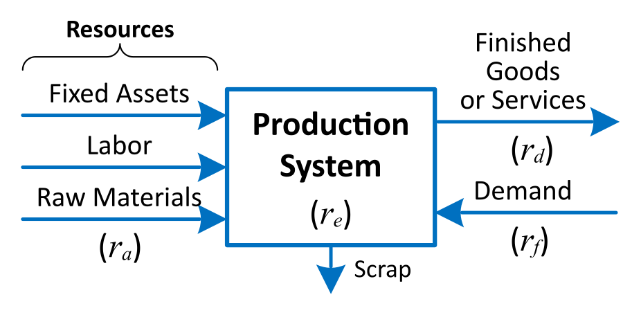
The production system in Fig. 1 is described by a set of rates (all in units q/t):
- r_e
- = effective production/service rate, the capacity of the production system
- r_a
- = input (arrival) rate of work \left\{\begin{array}{l}\text{raw material, for goods production}\\\text{accepted demand, for a service system}\end{array}\right.
- r_d
- = departure rate of demand satisfied by the production system
- r_f
- = offered demand, the rate of work presented to the system.
These rates satisfy r_a \ge r_d, with r_a = r_d if there is no yield loss (true for most service systems); the shortfall r_a - r_d is the yield loss, leaving the system as the scrap of Fig. 1. When the input is controlled, as in most of what follows, the system admits all offered demand and r_f = r_a; but offered demand can exceed what the system is able to admit, for example when raw material is limited, and then a decision arises over how much of it to take in (r_f \ge r_a), one left to later topics.5
3. Little’s Law
Approximation formulas for a production system’s cycle time are related to its throughput via Little’s Law:
WIP = TH \times CT, \qquad TH = \frac{WIP}{CT}, \qquad CT = \frac{WIP}{TH}, \tag{1}
where
- TH
- = throughput
- WIP
- = work-in-process
- CT
- = cycle time.
Each is an average over a production system: throughput is its output per time period, in units per hour or any other rate; work-in-process is the number of units of product it holds; and cycle time is the time each unit spends in it.
For a serial production system or routing, WIP is the inventory between the start and end points of the routing and CT is the average time from release of a job at the beginning of the routing until it reaches an inventory point at the end of the routing. Fig. 2 shows a graphical depiction of Little’s Law,6 where the throughput corresponds to the slope of the lines representing the cumulative number of arrivals and departures.
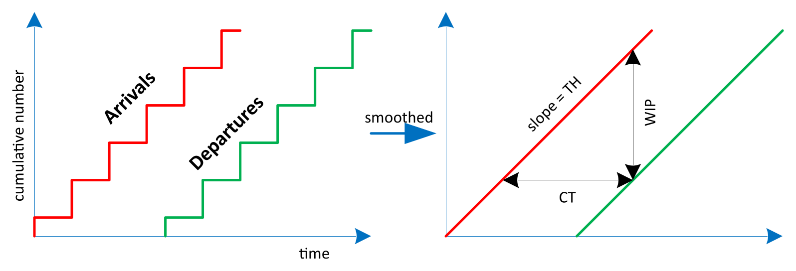
Given an existing production system, cycle time can be determined from WIP and TH by Little’s Law. When the production system does not yet exist and is just being designed, usually only a target throughput is known, while WIP and CT are unknown; cycle time can then be estimated (or simulated), and WIP determined from WIP = TH \cdot CT.
Example 2: Time in production
If the daily output of a production system is 25 units and the average number of units in process in the system is 50, what is the average amount of time each unit of product spends in production?
Major assumption: Little’s Law only applies in steady-state (stationary) situations; it does not work if TH, WIP, or CT are changing over time.
TH = 25 \text{ units/day}, \quad WIP = 50 \text{ units}, \quad CT = \frac{WIP}{TH} = \frac{50}{25} = 2 \text{ days}.
≈ 2 days in production
Example 3: Students in a department
If it takes, on average, nine semesters for an undergraduate IE student to graduate and there are, on average, 360 students in the department, how many students, on average, graduate each semester?
TH = \frac{WIP}{CT} = \frac{360}{9} = 40 \text{ graduates per semester}.
≈ 40 graduates per semester
Stock-vs-flow distinction. Both examples are the same statement about a stock and a flow. The work in process is a stock, the quantity accumulated inside a system’s boundary, and the throughput is a flow, the rate at which units cross that boundary. In Fig. 2 the flow is the slope of the cumulative curves and the stock is the vertical gap between them. Like water in a bathtub, a stock rises when its inflow outruns its outflow and holds steady only when the two balance, the steady state Little’s Law requires. Read this way, WIP = TH \times CT is the general identity stock = flow × time in system, and it reaches well beyond a factory floor: in Ex. 3 the students are the stock and the graduates per semester the flow. Little’s Law holds, in fact, for almost any system in steady state, under very weak assumptions.7
To find where it applies, look for three things:
- A boundary, a system that units enter and later leave.
- A stock, a countable quantity held inside it (jobs, patients, students, orders, inventory, even dollars).
- A flow, the rate at which units cross the boundary, with inflow and outflow in long-run balance.
Given those three, the average time a unit spends inside is the stock divided by the flow, CT = WIP / TH. The inventory in a warehouse (a stock) and the rate at which product ships from it (a flow), for instance, give the average time a unit sits in stock. The stock-and-flow distinction is the foundation of system dynamics.8
4. Variability and the Poisson process
Measuring variability
The squared coefficient of variation (SCV) provides a normalized measure used to estimate the variance of a process (demand, production, etc.):
\begin{aligned} c &= \frac{\sigma}{t}, \\ c^2 &= \frac{\sigma^2}{t^2}, \end{aligned} \tag{2}
where c is the coefficient of variation (CV), c^2 the squared coefficient of variation (SCV), \sigma the standard deviation of the process, t its mean, and \sigma^2 its variance. The SCV places a process on a scale of variability:
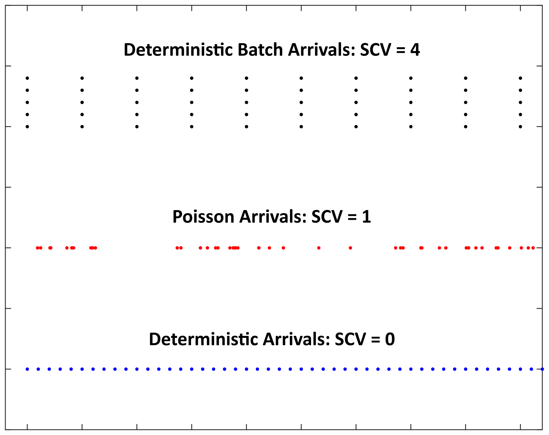
- c^2 = 0: deterministic / exactly spaced (best case, lower bound);
- c^2 < 0.75: low variability;
- 0.75 \le c^2 < 1.33: moderate variability;
- c^2 = 1: Poisson, i.e., totally random (practical worst case, upper bound);
- c^2 \ge 1.33: high variability (bad control).
All three arrival streams in Fig. 3 have the same rate of 10 per hour; they differ only in their SCV.
Totally random arrivals
When each short time interval carries the same small, independent chance of an arrival, the process appears completely random. For arrivals at an average rate r_a, the time between successive arrivals then follows the exponential distribution, whose mean is 1/r_a: at r_a = 5 customers per hour, an average gap of 12 minutes. The exponential is memoryless: however long it has been since the last arrival, the time remaining until the next one keeps the same distribution. The derivation, using a barber shop as the running example, is in the collapsed note below; it is optional background for the interested reader, and only the result is used in what follows.
NoteDerivation: totally random arrivals and the exponential distribution
Assume a barber shop is in a city of N = 10{,}000 people, and customers arrive at an average rate of r_a = 5 per hour. Divide time into short intervals of length \Delta t = 1 min, and suppose that in each interval every person in the city independently walks in with the same small probability p.
Matching the rate. With N people each arriving with chance p, the expected number of arrivals in one interval is Np. For the process to average r_a arrivals per hour, this expectation must equal r_a \Delta t, the average number of arrivals in a slice of time of length \Delta t. Setting the two equal pins down p:
Np = r_a \Delta t = 5 \cdot \tfrac{1}{60} = \tfrac{1}{12} \;\Rightarrow\; p = \tfrac{1}{12 \cdot 10{,}000} = \tfrac{1}{120{,}000} \ \text{chance of arrival per min per person.}
No arrival for a time t. Let T be the time from one arrival to the next. Because p is tiny, the chance that someone arrives during a given interval is approximately Np = r_a \Delta t (the chance of two or more arrivals in the same minute is negligible). The event T > t requires that no one arrive in any of the t/\Delta t consecutive intervals making up the gap, and since the intervals are independent, their no-arrival chances multiply:
\mathbb{P}(T > t) = (1 - Np)^{t/\Delta t} = (1 - r_a \Delta t)^{t/\Delta t} = \big[(1 - r_a \Delta t)^{1/\Delta t}\big]^t .
The last step only regroups the exponent: everything that depends on the interval width \Delta t is collected inside the brackets, with the elapsed time t outside.
Shrinking the interval. The one-minute interval was an arbitrary choice; the truly continuous random process is what remains as \Delta t \to 0. The bracketed factor then approaches a standard limit. Substituting x = r_a \Delta t, so that 1/\Delta t = r_a/x and x \to 0 as \Delta t \to 0, turns it into \big[(1-x)^{1/x}\big]^{r_a}, and the classic limit \lim_{x\to 0}(1-x)^{1/x} = e^{-1} gives
\left.\begin{array}{l} x = r_a \Delta t \Rightarrow \Delta t = x/r_a \\ \lim_{x\to 0}(1-x)^{1/x} = e^{-1}\end{array}\right\} \;\Rightarrow\; \lim_{\Delta t\to 0}(1 - r_a \Delta t)^{1/\Delta t} = \big(e^{-1}\big)^{r_a} = e^{-r_a} .
The exponential result. Raising the limit to the power t gives the survival probability of the inter-arrival time, and with it the mean:
\boxed{\mathbb{P}(T > t) = e^{-r_a t}}, \qquad \mathbb{E}[T] = \tfrac{1}{r_a} = \tfrac{1}{5} = 0.2 \ \text{hr} = 12 \ \text{min.} \tag{3}
This is the exponential distribution with rate r_a: at 5 customers per hour, the average gap between arrivals is 12 minutes. Nothing in e^{-r_a t} records how long it has already been since the last arrival, which is the memoryless property. Before taking the limit, the number of intervals until the next arrival followed a discrete geometric distribution; the exponential is its continuous limit as \Delta t shrinks.
This memoryless, totally-random pattern is the Poisson process, the c^2 = 1 reference on the scale above; Sec. 7 returns to these arrivals and reproduces their mean and SCV by simulation.
5. Throughput feasibility
The throughput requirement of each workstation corresponds to the desired output rate of nondefective units from the workstation, r_d. When using Little’s Law to determine the WIP at a workstation, the throughput to the workstation corresponds to the rate of units input to the workstation, r_a.
Increasing the departure rate to account for yield loss results in the required arrival rate to the station, r_a = r_d / y (with y the yield, the fraction of nondefective units produced).
The throughput-feasible minimum number of identical machines at the workstation is the fewest whose combined effective capacity (service rate) strictly exceeds that arrival rate. It is found by a machine-hours accounting, a general method of determining resource requirements (the resources can be machines, people, etc.) that can also be used to determine operating costs for economic justification. Over H hours of operation, the available machine hours mH split into processing, repair, and idle hours, and the minimum number of machines is the machine hours needed to meet demand divided by the productive hours per machine:
\begin{aligned} m_{\min} &= \left\lfloor \frac{\text{machine hours needed to meet demand}}{\text{productive hours per machine}} + 1 \right\rfloor \\ &= \left\lfloor \frac{r_a t_0 H}{AH} + 1 \right\rfloor = \left\lfloor r_a \frac{t_0}{A} + 1 \right\rfloor = \lfloor r_a t_e + 1 \rfloor , \end{aligned} \tag{4}
where
- r_a
- = arrival rate to workstation
- t_0
- = natural mean process time
- A
- = availability
- = \text{MTTF}/(\text{MTTF}+\text{MTTR})
- t_e
- = effective mean process time with failures
- = t_0/A
- H
- = hours of operation
- m
- = number of identical machines installed (m \ge m_{\min})
- r_e
- = service rate (effective capacity)
- = m/t_e
- \text{MTTF}
- = mean time to failure
- \text{MTTR}
- = mean time to repair.
The failures folded into t_e are preemptive outages: breakdowns that can strike while a job is in process, not only between jobs.
The word effective signals a deliberate device: two quantities folded into one workable number. Here the natural process time and the long-run availability are combined into a single effective process time.
Over those H hours the available machine hours split into processing, repair, and idle:
mH = \underbrace{r_a\,t_0\,H}_{\text{processing}} + \underbrace{r_a\,(t_e - t_0)\,H}_{\text{repair}} + \underbrace{(m - r_a\,t_e)\,H}_{\text{idle}} ,
so each machine supplies AH productive hours. (Using \lfloor r_a\,t_e \rfloor would not work, since r_a\,t_e could be an integer, which would result in a utilization of 100%.)
More machines than this minimum may be installed. A workstation is designed to run with its utilization strictly below one, a rule of design rather than a mere algebraic fact,
u = \frac{r_a}{r_e} = \frac{r_a\,t_e}{m} < 1 , \tag{5}
and every machine added beyond m_{\min} lowers the utilization u and, through the cycle-time relation of Sec. 6, shortens the cycle time. The condition u < 1 is a statement about the long-run average, not about every instant. Demand can outrun capacity in short bursts, and those bursts are what build the queue; the lulls that follow drain it. Only over the long run must the average stay below one.
The four-workstation line of Fig. 4 makes this concrete, and the same line is carried through to cycle time in Sec. 6.
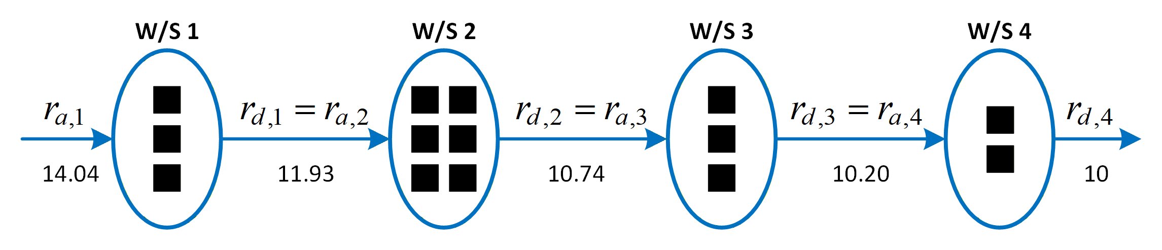
Table 1 shows the calculations used to determine the minimum number of machines necessary to produce a throughput of 10 parts per hour from this line (a throughput-feasible capacity plan). Working back from the required 10 good units/hr at the last station, each station’s arrival rate is its departure rate inflated by yield, r_a = r_d / y, and that arrival rate becomes the departure rate of the station upstream.
| W/S 1 | W/S 2 | W/S 3 | W/S 4 | |
|---|---|---|---|---|
| Arrival rate r_a (q/hr) | 14.04 | 11.93 | 10.74 | 10.20 |
| Natural process time t_0 (hr) | 0.20 | 0.50 | 0.25 | 0.15 |
| MTTF (hr) | 40 | — | 100 | — |
| MTTR (hr) | 2 | 0 | 5 | 0 |
| Availability A | 0.952 | 1 | 0.952 | 1 |
| Effective process time t_e (hr) | 0.21 | 0.50 | 0.2625 | 0.15 |
| Machines m | 3 | 6 | 3 | 2 |
| Utilization u | 0.983 | 0.995 | 0.940 | 0.765 |
| Yield y | 0.85 | 0.90 | 0.95 | 0.98 |
| Departure rate r_d (q/hr) | 11.93 | 10.74 | 10.20 | 10.00 |
NoteA yield paradox: lower yield, shorter cycle time
A counterintuitive consequence follows. Lowering a station’s yield raises the rate of units that must enter it, r_a = r_d / y. With work in process held fixed, Little’s Law confirms that the cycle time then falls rather than rises. The gain is not free: the higher input rate is met only by adding capacity, on the order of a third more at a yield of 0.75.
6. Level 2: Cycle-time estimation
Level 2 of the levels of modeling in Lecture 1.1 Sec. 4, the nonlinear one that brings in variability, is reached here. The following queuing approximation formulas estimate the cycle time of a single-machine workstation (G/G/1)9 or a workstation with m identical machines (G/G/m); when m = 1, the G/G/m equation reduces to the G/G/1 equation. The cycle time splits into queuing time plus process time, and the queuing time is the product of a variability factor, a utilization factor, and the process time (the VUT form):
\boxed{\,t_{CT} = \underbrace{t_{CT_q}}_{\text{queuing time}} + \underbrace{t_e}_{\text{process time}} = \underbrace{\left(\frac{c_a^2 + c_e^2}{2}\right)}_{\text{variability}} \underbrace{\left(\frac{u}{1-u}\right)}_{\text{utilization}} \underbrace{\,t_e\,}_{\text{time}} + t_e\,} \tag{6}
For m identical machines the utilization factor generalizes; the departure SCV of one station becomes the arrival SCV of the next, and the effective process-time SCV folds in machine failures:
\hphantom{\underset{\displaystyle \text{Eff. process time SCV:}}{\underset{\displaystyle \text{Departure SCV:}}{\text{G/G/}m:}}}\mathllap{\text{G/G/}m:}\quad \hphantom{\underset{\displaystyle c_e^2}{\underset{\displaystyle c_d^2}{t_{CT_q}}}}\mathllap{t_{CT_q}} = \mathrlap{\left(\frac{c_a^2 + c_e^2}{2}\right)\frac{u^{\sqrt{2(m+1)}-1}}{m\,(1-u)}\,t_e ,}\hphantom{\underset{\displaystyle c_0^2 + (1 + c_r^2)\,A(1-A)\,\frac{\text{MTTR}}{t_0} ,}{\underset{\displaystyle 1 + (1-u^2)(c_a^2 - 1) + \frac{u^2}{\sqrt{m}}\,(c_e^2 - 1) ,}{\left(\frac{c_a^2 + c_e^2}{2}\right)\frac{u^{\sqrt{2(m+1)}-1}}{m\,(1-u)}\,t_e ,}}} \tag{7}
\hphantom{\underset{\displaystyle \text{Eff. process time SCV:}}{\underset{\displaystyle \text{Departure SCV:}}{\text{G/G/}m:}}}\mathllap{\text{Departure SCV:}}\quad \hphantom{\underset{\displaystyle c_e^2}{\underset{\displaystyle c_d^2}{t_{CT_q}}}}\mathllap{c_d^2} = \mathrlap{1 + (1-u^2)(c_a^2 - 1) + \frac{u^2}{\sqrt{m}}\,(c_e^2 - 1) ,}\hphantom{\underset{\displaystyle c_0^2 + (1 + c_r^2)\,A(1-A)\,\frac{\text{MTTR}}{t_0} ,}{\underset{\displaystyle 1 + (1-u^2)(c_a^2 - 1) + \frac{u^2}{\sqrt{m}}\,(c_e^2 - 1) ,}{\left(\frac{c_a^2 + c_e^2}{2}\right)\frac{u^{\sqrt{2(m+1)}-1}}{m\,(1-u)}\,t_e ,}}} \tag{8}
\hphantom{\underset{\displaystyle \text{Eff. process time SCV:}}{\underset{\displaystyle \text{Departure SCV:}}{\text{G/G/}m:}}}\mathllap{\text{Eff. process time SCV:}}\quad \hphantom{\underset{\displaystyle c_e^2}{\underset{\displaystyle c_d^2}{t_{CT_q}}}}\mathllap{c_e^2} = \mathrlap{c_0^2 + (1 + c_r^2)\,A(1-A)\,\frac{\text{MTTR}}{t_0} ,}\hphantom{\underset{\displaystyle c_0^2 + (1 + c_r^2)\,A(1-A)\,\frac{\text{MTTR}}{t_0} ,}{\underset{\displaystyle 1 + (1-u^2)(c_a^2 - 1) + \frac{u^2}{\sqrt{m}}\,(c_e^2 - 1) ,}{\left(\frac{c_a^2 + c_e^2}{2}\right)\frac{u^{\sqrt{2(m+1)}-1}}{m\,(1-u)}\,t_e ,}}} \tag{9}
where
- u
- = utilization
- = r_a\,t_e / m
- c_a^2
- = arrival SCV
- = \sigma_a^2 / t_a^2
- t_a
- = mean time between arrivals
- = 1/r_a
- c_e^2
- = effective process-time SCV with failures
- c_0^2
- = natural process-time SCV
- = \sigma_0^2 / t_0^2
- c_r^2
- = repair-time SCV
- = \sigma_r^2 / \text{MTTR}^2.
For the arrival SCV, \sigma_a^2 = 0 for deterministic arrivals and \sigma_a^2 = t_a^2 for exponential ones.
The single-machine form Eq. 6 is Kingman’s approximation, named for this lecture’s epigraph author; the m-machine results (Eq. 7, Eq. 8, Eq. 9) are further factory-physics formulas, quoted here rather than derived. These formulas are checked against a simulation in Sec. 7, where simulation is introduced as a modeling level in its own right.
Example 4: Price of utilization
How does the cycle time of a single-machine station (t_e = 0.1 hr, c_a^2 = c_e^2 = 1) behave as utilization rises toward 1?
Cycle time climbs gently and then explodes as the station nears full load (Fig. 5): the last increment of utilization is by far the most expensive, which is why a system is rarely designed to run flat out.
Utilization is deceptively benign until it is not: little changes up to about 70 percent, then the queue climbs steeply as it nears 100 percent. The factor u/(1-u) is the reason, its denominator shrinking toward zero as u \to 1, and the growth runs well outside everyday intuition, a rise from 0.8 to 0.9 can triple the cycle time.
Continuing with the throughput-feasible plan of Sec. 5, Table 2 estimates the cycle time of the line and the total cost of its machines. The arrival rate r_a is used to calculate the WIP (instead of the throughput TH = r_d), due to the conservative assumption that all failures are identified at the end of processing. A scrapped unit then costs twice: the raw material is lost, and the machine time spent on it is lost as well. Moving inspection upstream recovers the wasted capacity, but only where utilization is high; where a station is lightly loaded there is little to recover, since the same material is discarded either way. The station SCV inputs enter as given data: the first station sees Poisson arrivals (c_a^2 = 1), and each station’s natural-process SCV c_0^2 and repair-time SCV c_r^2 are specified with the plan.
| W/S 1 | W/S 2 | W/S 3 | W/S 4 | Total | |
|---|---|---|---|---|---|
| Arrival SCV c_a^2 | 1.0 | 1.088 | 0.597 | 0.906 | |
| Natural process SCV c_0^2 | 0.25 | 0.0 | 0.0 | 0.5 | |
| Eff. process SCV c_e^2 | 1.157 | 0.0 | 0.907 | 0.5 | |
| Departure SCV c_d^2 | 1.088 | 0.597 | 0.906 | 0.754 | |
| Cycle time in queue CT_q (hr) | 4.265 | 8.191 | 0.977 | 0.152 | 13.585 |
| Cycle time CT (hr) | 4.475 | 8.691 | 1.239 | 0.302 | 14.707 |
| WIP at W/S | 62.83 | 103.72 | 13.31 | 3.09 | 182.95 |
| W/S cost ($000) | 36 | 108 | 6 | 12 | 162 |
Workstation 2 dominates the line: its 0.995 utilization drives by far the longest queue, the bottleneck a redesign would attack first.
Example 5: Pizza delivery time
The pizza shop whose delivery area was sized in Ex. 4 in Lecture 1.1 runs m delivery drivers against Poisson demand. How long does a customer wait from order to delivery, and how does that depend on the number of drivers?
Treat each driver as a machine and the shop as an m-machine station: a pizza is a job, a driver out on a run is a busy machine, and an order with no free driver waits in queue. The cycle time of Eq. 7 is then exactly the average order-to-door time. Three inputs fix it:
- Service time. From Ex. 4 in Lecture 1.1 a round trip averages \tfrac{4}{3}R = 4 mi; at an average 24 mph that ties up one driver for t_e = 4/24 = \tfrac{1}{6} hr \approx 10 min per delivery (one pizza at a time).
- Demand. Orders arrive Poisson at r_a = 20/hr (a busy evening), so c_a^2 = 1.
- Service variability. Delivery times vary with distance; take c_e^2 = 1 as a simple approximation.
The offered load is r_a t_e = 20\cdot\tfrac{1}{6} \approx 3.33 driver-hours of work per hour, so the throughput-feasible minimum (Eq. 4) is m_{\min} = \lfloor r_a\,t_e + 1 \rfloor = 4 drivers, the fewest that keep the utilization below one (u = r_a t_e / m < 1). Table 3 evaluates Eq. 7 across driver counts from this minimum upward.
| drivers m | utilization u | queue wait (min) | delivery time (min) |
|---|---|---|---|
| 4 | 0.833 | 10.1 | 20.1 |
| 5 | 0.667 | 2.2 | 12.2 |
| 6 | 0.556 | 0.7 | 10.7 |
| 7 | 0.476 | 0.3 | 10.3 |
| 8 | 0.417 | 0.1 | 10.1 |
With only m_{\min} = 4 drivers the shop runs at u = 0.83, and a customer waits about as long in queue as the drive itself takes: roughly 20 minutes door to door, half of it spent waiting for a driver to come free. Each added driver cuts that queue sharply: a fifth driver nearly halves the total time, and past m = 6 the wait is negligible and the delivery time is essentially the drive. This is the lesson of Fig. 5 again, that the last increment of utilization is the costly one, now answering an operational question the distance estimate of Lecture 1.1 could not: with high demand and too few drivers, the wait, not the drive, dominates.
7. Level 3: Simulation
The remaining level of modeling from Lecture 1.1 Sec. 4 is level 3: simulation, and this is its first appearance in the course. A simulation model does not solve a system; it plays the system out, with random draws standing in for whatever the model treats as random. Among the levels, level 3 is the tool for complex interactions, behavior beyond the reach of any closed-form formula. It is equally the tool for behavior that never settles down: the queueing formulas above are all long-run averages, and a system that never leaves its start-up transient has no closed-form estimate at all, so simulation is the only recourse (Sec. 8). It is introduced here on problems the earlier levels have already solved, deliberately: a simulation checked against a known answer can then be trusted on questions that have none.
The simplest form is Monte Carlo simulation: draw random samples and read statistics off them, with no clock and no system state. Model 1 generates the totally random arrivals of Sec. 4 by drawing each inter-arrival time as -\ln(U)/r_a from a uniform U, a use of inverse-transform sampling: inverting the exponential’s cumulative distribution turns independent uniforms into exponential gaps.
The models from here on are written at two depths, and the boxes are labelled accordingly. A model stated in words alone, in the keyword form of Lecture 1.1, is the concept, and it is captioned with the model’s number and name and nothing else, because the concept is what a model is. Committing that statement to runnable Julia is the implementation, captioned “Model N implementation” so it is clear which concept it belongs to. A third depth, the formulation, sits between them when a model is worth writing in symbols before it is written in code; these first models go straight to Julia and so have none. Descending is meant to add detail without changing what the depth above said, which is why the two are shown separately rather than merged: a constraint that appears in the code and nowhere in the concept is something determined silently.10
NoteInverse-transform sampling: turning uniforms into any distribution
A computer supplies uniform random numbers on [0,1]; inverse-transform sampling turns them into draws from any distribution with a known cumulative distribution function (CDF) F. To sample a value X whose CDF is F, draw U uniform on [0,1] and invert:
X = F^{-1}(U).
This works because, for uniform U,
\mathbb{P}(X \le x) = \mathbb{P}\!\big(F^{-1}(U) \le x\big) = \mathbb{P}\!\big(U \le F(x)\big) = F(x),
so X carries exactly the target CDF F.
For the exponential inter-arrival time of Sec. 4, the CDF is F(t) = 1 - e^{-r_a t} (from the survival result \mathbb{P}(T > t) = e^{-r_a t} derived there). Setting u = 1 - e^{-r_a t} and solving for t gives
t = -\frac{\ln(1 - u)}{r_a}.
Because 1 - U is itself uniform on [0,1], it may stand in for U, leaving the form used in the code, t = -\ln(U)/r_a (-log(rand()) / rₐ).
The method is standard for random-variate generation; see A. M. Law and W. D. Kelton, Simulation Modeling and Analysis, 2nd ed. (McGraw-Hill, 1991), Sec. 8.2.1.
return: sample of n inter-arrival times from a Poisson stream at rate r_a
assumptions:
(a) inter-arrival times are independent exponential draws at rate r_a;
(b) rate r_a is constant over the run (homogeneous).
Model 1 implementation: Poisson arrival simulation
Drawing the times and reading back their mean and SCV recovers the analytic values of Sec. 4:
(0.20010545354252723, 1.0050114030765351)A production system needs more than samples: in discrete-event simulation the state of the system updates event by event, and performance is read off the simulated history the way it would be measured on the real system. A short single-server simulation confirms the G/G/1 form. Model 2 plays a first-in-first-out queue out job by job with the Lindley recursion (each job waits behind whatever work is left when it arrives), and its simulated mean cycle time matches Eq. 6. For this M/M/1 station that estimate is exact: t_{CT} = \frac{u}{1-u}t_e + t_e = \frac{0.8}{0.2}(0.1)+0.1 = 0.5 hr, equivalently 1/(r_e - r_a) = 1/(10-8) = 0.5 hr, so the run below has a known target of 0.5 to reproduce. The recursion is the single line wq = max(0, wq + s - a): the work wq a job finds waiting is its queue delay, and after its service s is added and the gap a to the next arrival subtracted, the floor at zero empties the queue whenever an arrival finds the server free.
return: cycle time of each job through a single-server FIFO queue
assumptions:
(a) exponential inter-arrivals at rate r_a and exponential service at mean t_e, so c_a^2 = c_e^2 = 1;
(b) one server, first-in-first-out, one job at a time;
(c) queue starts empty.
Model 2 implementation: Single-server queue simulation
# Model: single-server FIFO queue simulation
function queue(rₐ, tₑ, n)
ct = zeros(n) # cycle time of each job
wq = 0.0 # work waiting when a job arrives
for i in 1:n
s = -tₑ * log(rand()) # exponential service time
ct[i] = wq + s # cycle time = wait + service
a = -log(rand()) / rₐ # gap to the next arrival
wq = max(0.0, wq + s - a) # Lindley recursion
end
return ct
endqueue (generic function with 1 method)(0.5379312820032124, 0.5000000000000001)
One run is one draw. The convergence in Fig. 6 is a single run: one seed, one stream of random draws, one simulated history. A different seed produces a different history whose average lands somewhere else, so a single run, however long, is one noisy estimate of the long-run mean. The remedy is a simulation experiment: several independent replications, averaged. The spread across replications shows how much any single run can be trusted, and the grand mean, reported with a 95% confidence interval, brackets the known analytic value of 0.5:
# Code block 3: twenty replications and a confidence interval
Random.seed!(2)
nrep = 20 # independent replications
njob = 1_000_000 # jobs per replication
reps = [sum(queue(8, 0.1, njob)) / njob for _ in 1:nrep]
grand = sum(reps) / nrep # grand mean over the experiment
se = sqrt(sum((reps .- grand).^2) / (nrep*(nrep - 1)))
ci = 1.96 * se # 95% confidence half-width
(grand, ci, vut) # grand mean, half-width, target 0.5(0.5013803714212831, 0.0019566048839431897, 0.5000000000000001)The trade. The two levels complement each other. The level-2 formula delivers the long-run average instantly, one line of arithmetic, with its assumptions in plain sight. The simulation spends millions of simulated jobs to approach the same number, and tighter precision costs more replications still. For the long-run average of a standard queue, the formula is the right tool. The simulation earns its keep in the other direction: change the system in a way the formula cannot express, and the model needs only a few edited lines. The formula gives speed on the questions it can pose; the simulation gives reach on the questions it cannot; where they overlap, each checks the other.
Both Eq. 6 and Model 2 assume first-in-first-out service. Nothing in a real queue requires that. A workstation might instead serve the shortest waiting job first (shortest processing time, SPT), expediting quick jobs at the expense of long ones. The VUT equation has no term for queue discipline, and extending the level-2 analysis to one is hard to impossible; in the simulation, the discipline is just the rule for choosing which waiting job goes next. Model 3 replays the same station with that one rule changed.
return: cycle time of each job through a single-server queue that serves the shortest waiting job first
assumptions:
(a) exponential inter-arrivals at rate r_a and exponential service at mean t_e, so c_a^2 = c_e^2 = 1;
(b) one server, non-preemptive: a job in service finishes before the next choice is made;
(c) queue starts empty.
Model 3 implementation: Single-server SPT queue simulation
# Model: single-server SPT queue simulation
function queue_spt(rₐ, tₑ, n)
at = cumsum([-log(rand()) / rₐ for _ in 1:n]) # arrivals
st = [-tₑ * log(rand()) for _ in 1:n] # service times
ct = zeros(n) # cycle time of each job
pend = Int[] # jobs waiting for the server
t, i = 0.0, 1 # clock, next arrival index
for _ in 1:n
while i ≤ n && at[i] ≤ t # arrivals up to time t
push!(pend, i); i += 1
end
if isempty(pend) # idle: jump to next arrival
t = at[i]; push!(pend, i); i += 1
end
j = argmin(k -> st[k], pend) # shortest job next
filter!(k -> k ≠ j, pend)
t += st[j] # serve job j to completion
ct[j] = t - at[j] # cycle time = finish - arrival
end
return ct
endqueue_spt (generic function with 1 method)(0.4903948204599785, 0.2923649598218)The loop keeps an explicit clock t and a list pend of jobs that have arrived but not yet been served: each pass admits every arrival up to the clock, jumps the clock to the next arrival when the server is idle, then argmin selects the shortest pending job, filter! removes it, and the clock advances by that job’s service time. Serving the shortest job first cuts the mean cycle time well below the FIFO value: the same jobs, the same utilization, the same variability, only the order of service changed. The level-2 formula cannot see this lever at all; for the level-3 model it is one line. The stationarity question of Sec. 8, what happens when a queue never runs long enough to reach its long-run average, is the same story again: outside the formula’s reach, directly answerable by simulation.
8. Stationarity
The cycle-time estimate also assumes the demand process is stationary: its statistics do not drift over the horizon, so the estimate is a long-run average. Trend, seasonality, or a one-time structural change all break this, the same conditions under which the mean stops being scalable (mean-value analysis, Lecture 1.1). A non-stationary series must first be made stationary. Fig. 7 takes each of those violations out in turn, and the series to carry forward is the one left at the end: the estimate is entitled to that series, not to the one first observed.
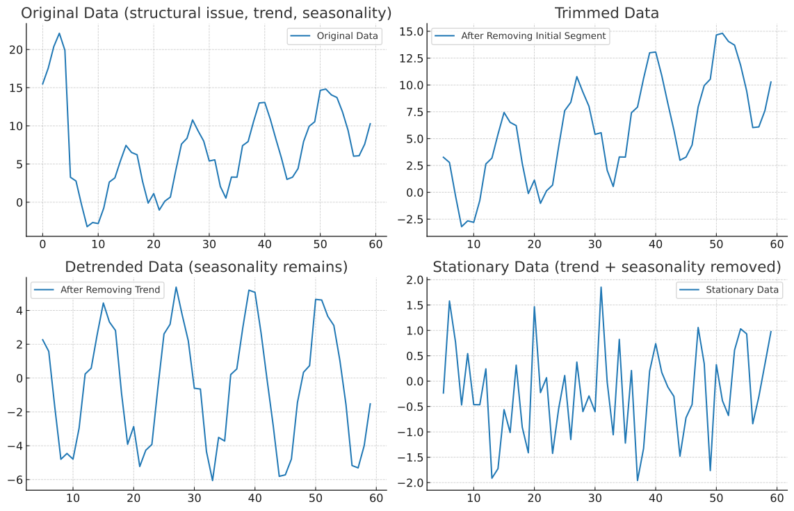
The same caveat shows up operationally. A goods-producing system carries work in process from shift to shift and, run long enough under stationary demand, approaches the steady-state averages the VUT formula reports; many service systems do not, clearing every day and starting each morning empty, so a short enough day is spent entirely in the start-up transient, where the steady-state estimate does not apply and simulation is the only recourse. This is the transient case Sec. 7 raised as a first-class reason to simulate. A barber shop open around the clock (8,760 hours per year) is stationary; one open only 10 hours a day is not, and there is little customer waiting at the start of each day even when utilization is high. A customer arrival rate that varies throughout the day is likewise nonstationary, and can be modeled with a nonhomogeneous Poisson process, using, for example, a different arrival rate each hour.
A short simulation of the barber shop (r_e = 6/hr, c_e^2 = 0, a deterministic 10-minute cut) makes the point (Table 4). Run around the clock for a full year (8,760 hr), the simulated cycle time in queue matches the steady-state estimate of Eq. 6; run only 10 hours a day, the queue never leaves its start-of-day transient and the average wait falls well short of the steady-state value, the more so the higher the utilization. Fig. 8 traces the same shortfall continuously: the simulated wait climbs toward the steady-state estimate only as the daily hours grow, a ten-hour service day reaching barely seventy percent of it.
| r_a | r_e | nruns | nhrs | u | CT_q sim | CT_q est | sim/est | |
|---|---|---|---|---|---|---|---|---|
| 1 | 5 | 6 | 1 | 8760 | 0.8333 | 0.41 | 0.4167 | 0.984 |
| 2 | 5 | 6 | 500 | 8760 | 0.8333 | 0.4166 | 0.4167 | 0.9998 |
| 3 | 5 | 6 | 500 | 10 | 0.8333 | 0.2723 | 0.4167 | 0.6536 |
| 4 | 4 | 6 | 500 | 10 | 0.6667 | 0.1407 | 0.1667 | 0.8442 |
| 5 | 2 | 6 | 500 | 10 | 0.3333 | 0.0375 | 0.0417 | 0.8992 |

9. Where variability goes in a line
The departure SCV (Eq. 8) means a station’s variability does not stay put: the variability of what leaves one station becomes the variability of what arrives at the next. A highly variable station placed early inflates the queue of every station downstream, while the same station placed last corrupts nothing beyond itself. This is the corrupting influence of variability: variability early in a line is far more damaging than variability late. When the order of operations is a design choice, that choice matters.
Example 6: Variable station placement
Three single-machine stations run in series, each at utilization u = 0.9 and the same mean process time t_e = 0.1 hr, but with process-time variabilities c_e^2 = 0.25, 1, and 4; work enters the first at c_a^2 = 1. Compare the line’s total cycle time when the most variable station is run last versus first.
# Code block 5: station order and its effect on cycle time
u = 0.9 # utilization at each station
tₑ = 0.1 # hr, same mean process time
for order in ([0.25, 1, 4], [4, 1, 0.25])
CT = let c²ₐ = 1.0, total = 0.0
for c²ₑ in order
CTq = (c²ₐ + c²ₑ)/2 * u/(1 - u) * tₑ
total += CTq + tₑ # station cycle time
c²ₐ = (1 - u^2)*c²ₐ + u^2*c²ₑ # to next (eq-cd)
end
total
end
@show order, CT
end(order, CT) = ([0.25, 1.0, 4.0], 3.6871837500000013)
(order, CT) = ([4.0, 1.0, 0.25], 5.313765)The most-variable-last ordering carries about a third less total cycle time. The line carrying each station’s SCV to the next, c_a^2 \leftarrow (1-u^2)c_a^2 + u^2 c_e^2, is Eq. 8 at m = 1, where \sqrt{m} = 1 and the constant terms cancel. The rule: put low-variability operations early and the most variable operation last, and invest variability-reduction effort upstream, where it pays off across every stage that follows. Once supply chains are introduced (from Topic 2 on), the same machinery answers where in a multi-stage chain to place the most variable activity.
Endnotes
“The First Erlang Century—and the Next,” Queueing Systems 63 (2009), p. 7.↩︎
The self-equalizing-headway method is due to John J. Bartholdi III and Donald D. Eisenstein, “A self-coördinating bus route to resist bus bunching,” Transportation Research Part B 46(4):481–491, 2012, implemented at Georgia Tech as the Tech Trolley real-time system (http://www.nextbuzz.gatech.edu/).↩︎
Hopp, W.J., and Spearman, M.L., 2000, Factory Physics: Foundations of Manufacturing Management, 2nd Ed., McGraw-Hill.↩︎
Suri, R., Sanders, J.L., and Kamath, M., 1993, “Performance evaluation of production networks,” Handbooks in OR & MS, vol. 4, S.C. Graves et al., Eds., pp. 199–286.↩︎
Cachon, G., and Terwiesch, C., 2006, Matching Supply with Demand: An Introduction to Operations Management, McGraw-Hill. The gap between offered demand and realized flow appears there as flow rate equal to the minimum of the demand rate and the process capacity, with a process accordingly termed demand-constrained or capacity-constrained.↩︎
The figure is adapted from Fig. 1.1 in Taylor and Karlin (1998).↩︎
John D. C. Little and Stephen C. Graves, “Little’s Law,” in D. Chhajed and T. J. Lowe, eds., Building Intuition: Insights from Basic Operations Management Models (Springer, 2008), 81–100.↩︎
John D. Sterman, Business Dynamics: Systems Thinking and Modeling for a Complex World (Irwin/McGraw-Hill, 2000).↩︎
In Kendall’s notation A/B/c, the three fields are the interarrival-time distribution, the service-time distribution, and the number of servers: M is Markovian (exponential, i.e., Poisson arrivals), D is deterministic (constant), and G is general (any distribution). So G/G/1 is a single server with general arrivals and service, M/M/1 has exponential arrivals and service, and M/D/1 has exponential arrivals with deterministic service.↩︎
The full form, including how competing approaches under one concept are labelled, is in the Model Format Reference.↩︎