3.2: One-Time Truck Shipments

ISE 754: Logistics Engineering, Fall 2026

If a carrier offers a price for a shipment, you cannot know whether it is reasonable unless you have estimated it yourself.

No new Julia packages used.

New Logjam functions used

• charge_ltl: Calculate LTL transport charge (rate × weight × distance, or minimum charge).
• charge_tl: Calculate TL transport charge (combining distance cost and minimum charge).
• maxpayld: Determine maximum payload limited by weight or cube capacity.
• mincharge_ltl: Calculate LTL minimum charge.
• mincharge_tl: Calculate TL minimum charge (independent of distance).
• rate_ltl: Estimate LTL (less-than-truckload) transportation rate.

Companion script

3-tran-2.jl, runnable Julia extracted from the lecture’s code blocks. (ppi-trucking.csv, the Producer Price Index snapshot Sec. 2.8 reads.)

1. Trucking services and operations

Lecture 3.1 ended where the transport rate becomes the question. Location worked with one monetary weight per facility and took the rate as given; transport works lane by lane, and a rate in dollars per ton-mile is what connects a flow in tons per year to a cost in dollars per mile. This lecture determines that rate for the one mode a logistics engineer needs to know in detail, and it does so for a shipment whose size is already known.

Trucking is the only transport mode that most shippers need to have detailed knowledge of. Only trucks are used for shipping and receiving at most facilities, and it is trucks that transport from facility to railhead, port and airport. Other modes are handled by specialized freight brokers.

1.1 For-hire services

Freight can be transported via private trucking or for-hire trucking. For-hire trucking services include full truckload (TL), less-than-truckload (LTL), and package express (PX), shown in Table 1. TL is 80% of all trucking.¹ PX can also include transport by rail and air, and it also has a limit on the maximum dimension of a load (e.g., 130 in.) in order to allow automated sortation equipment to be used at terminals. “Parcels” are PX loads, while loads under 2 lbs. are referred to as “packets.” Other services include bulk, motor vehicle carrier, refrigerated, and tank car.

Table 1: U.S. for-hire trucking services.

	TL	LTL	PX
Minimum payload	10,000 lb	150 lb	2 lb
Average payload	30,000 lb	1,000 lb	10 lb
Maximum payload	50,000 lb	10,000 lb	70 (UPS) – 150 lb
Average length of haul	294 mi	752 mi	894 mi
Average value	$775/ton	$7,002/ton	$37,538/ton

The two cutoffs in the first row are practice rather than regulation. Truckload is not usually considered unless at least 10,000 lb is being shipped, which is five tons. At the other end there is no strict physical cutoff for LTL: practically speaking, a shipment under 150 lb goes package express, and that is the minimum an LTL carrier’s own site will quote. Carriers such as FedEx now offer all three services, so the choice between them is a choice of product rather than of company.

The average value of an LTL load is nine times that of a TL load. The kind of product this course analyzes is the LTL kind, shipped in TL quantities.

The two haul lengths invite a question whose answer is about the statistic rather than about trucking. The average haul is 294 mi for TL and 752 mi for LTL, the reverse of what the payloads suggest. Nothing about a load changes at 10,000 lb. What the TL figure includes is truckloads of gravel, cement and similar bulk material, which are almost always shipped TL and almost always shipped a short distance, and those short hauls are averaged into the 294. The same mixing depresses the average value, since a great deal of very cheap and very heavy material moves TL. Both TL statistics are averages over a spectrum containing two quite different populations, and neither describes the general merchandise this course is about.

The maximum gross weight limit of 80,000 lbs applies to the entire vehicle (i.e., 3-axle tractor and 2-axle 53′ semi-trailer). The maximum payload weight of 50,000 lbs is based on an estimated average “tare” weight for the empty vehicle of approximately 30,000 lbs² (13,900 lb tractor and 13,800 lb semi-trailer). Although the physical cube capacity of a trailer ranges from 3,332 to 3,968 ft³ for 48 to 53 ft trailers, respectively, in practice not all of this space can be utilized when different-size items are packed into the trailer, resulting in an effective cube capacity from approximately 2,500 to 3,000 ft³.

Figure 1: The enclosed van semi-trailer, with interior dimensions in parenthesis.

Fig. 1 is where the two capacities this lecture uses most come from: 25 tons of payload and the cube the trailer encloses.

Three of the trailer’s four limits are set by regulation rather than by engineering. Width is capped because a lane is only so wide. Height is capped because a trailer has to pass under bridges. Weight is restricted per axle so the roadway is not damaged, which is what the weigh stations on an interstate are checking. Only length has moved: about thirty years ago the maximum went from 48 to 53 ft, and that five-foot extension took four or five years of monthly negotiation among every party with an interest in it.

NoteWhy a trailer advertises air ride on its side

The sign is not a comfort claim. On steel springs a trailer rises five or six inches when it is unloaded, so it has to be built short enough to clear a bridge at that raised height. Air suspension bleeds off pressure as the load comes out, holding a constant height, which lets the trailer be built deeper. The five or six inches that buys, over the whole floor area, is cube capacity, and Sec. 3.1 shows that cube capacity is usually what binds.

1.2 Routing and terminal networks

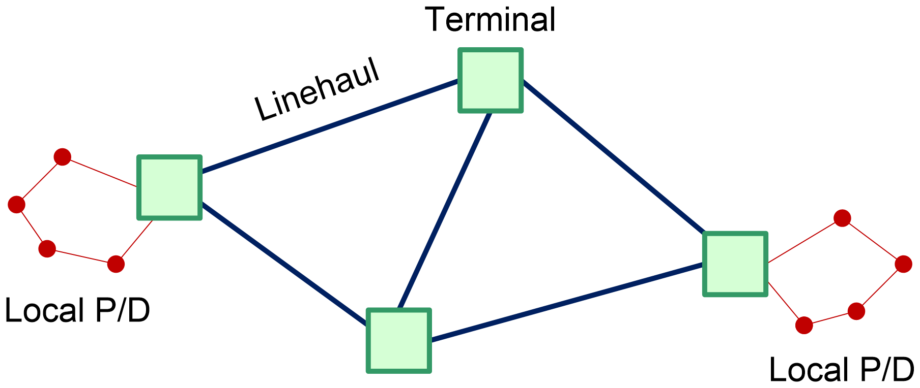
The routing alternatives available for TL trucking operations differ in how many pickups and deliveries a single truck makes. The major difference between TL and LTL/PX trucking operations is that the latter requires a network of terminals. In a LTL logistics network, loads in the vicinity of a terminal are collected and delivered to the terminal where they are sorted and loaded onto trucks that provide “linehaul” transport to other terminals. There are fewer firms providing LTL as compared to TL services because of the high cost of constructing a network of terminals. Non-revenue-generating empty (or “deadhead”) travel represents approximately 15% of total trucking miles and is used to reposition a tractor-trailer after the final delivery to the next initial pickup point.

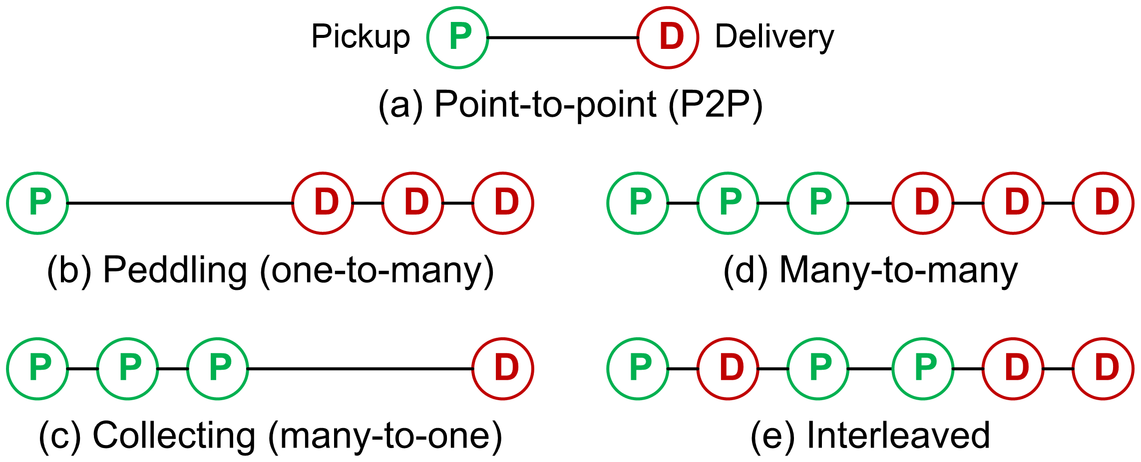
P2P abbreviates point to point: the truck picks up a load and does nothing else except deliver it at its destination, which is the simplest case to deal with. Peddling is multiple deliveries from a single pickup; collecting is many pickups to one delivery; many to many does all the pickups and then all the deliveries; interleaved mixes them.

Figure 2: The five TL routing alternatives. P is a pickup and D is a delivery.

Fig. 2 sets the five side by side, and reading (d) against (e) is what makes the next paragraph’s point visible. Interleaved routing (e) can be difficult to achieve if the trailer only opens at the rear.

Interleaved routing looks like the same operation as many-to-many, and the difference is physical rather than geometric. Most trailers load from the back, so under interleaving an early-delivered item can end up behind later ones and the driver spends time unloading freight only to reload it. A furniture moving truck has doors along its side for exactly this reason, so several households can be carried without one blocking another. The practical question that follows is how far a driver would be willing to drive out of the way to avoid unloading to reach the back, and good routing software answers it by considering how the truck is actually loaded rather than the route alone.

As compared to a single shipment transported from its origin to its destination (P2P TL), all of the multi-stop TL routing alternatives represent the consolidation of multiple shipments into a single consolidated load. The benefit of consolidation is the potential savings that may accrue from economies of scale in transportation gained by shipping larger loads. Consolidated truckloads can be used to transport loads that are smaller than P2P TL and that are of lesser value than LTL.

An LTL shipment is typically one or two pallets where a truckload is eighteen or twenty, so it is collected on a smaller vehicle, taken to a terminal, moved between two or three terminals, and then put out for delivery. Each trip between terminals is the linehaul, and it is separate from the local pickup and delivery at either end. The arrangement is the one the postal system uses.

Figure 3: The logistics network used for LTL and PX. Local pickup and delivery at each end, linehaul between terminals.

Fig. 3 is what a TL operation does not need, and the cost of building one is why there are far fewer LTL carriers than TL carriers.

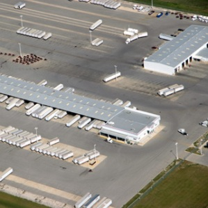
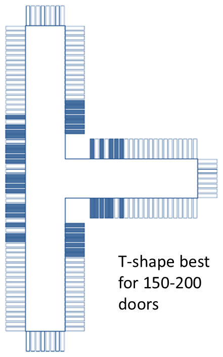
An LTL terminal is easy to mistake for a warehouse, and what distinguishes it is its shape. A warehouse on the same site would be far larger and would occupy the parking area; an LTL terminal is deliberately narrow, because it is not storing anything. Freight comes off one trailer and is carried across the building on a pallet jack to another. It is a switching network rather than a store, and a T-shape is the best shape at 150 to 200 doors, which is what Fig. 4 shows.³

Figure 4: An LTL terminal from the air, and the T-shape that is best at 150 to 200 doors.⁴ It is built long and narrow because nothing is stored in it: freight crosses from an inbound door to an outbound door, and the shape keeps that crossing short.

1.3 Hours of service

The Federal Motor Carrier Safety Administration’s Hours-of-Service (HOS) regulations provide constraints on the number of hours that a driver can operate a truck: “Drivers may drive up to 11 hours in the 14-hour on-duty window after they come on duty following 10 or more consecutive hours off duty.”⁵ The HOS regulations effectively limit the total distance traveled by a single driver in a day to around 400 miles. As a result, a DC is limited to serving customers located within a 200 mile radius if it is desired that drivers return to a home location each day. Similar considerations result in a 200-mile maximum separation between LTL terminals. Team drivers can be used to allow almost continual operation, where each driver must rest at least eight consecutive hours in the sleeper berth per HOS regulations.

The 400-mile day is why the 250-mile threshold in Sec. 2 matters: inside it a driver can deliver and return the same day.

The rule reaches further into logistics decisions than a safety regulation usually does, and a relay operation shows why. A service running out of the Port of Wilmington takes loads as far as North Augusta, Georgia, drops the trailer, and hands it to a second driver for the leg to Atlanta or Savannah. The first leg is under 250 miles, so it can be driven, dropped and driven back inside a ten-hour day, and the driver is home every night. Long-haul trucking has high turnover for the obvious reason, so an operation that can offer a normal day retains drivers that an over-the-road operation cannot.

1.4 One-time and periodic shipments

One-time shipments are an operational decision, and they are what this lecture is about: the shipment size q is known. A shipper already knows when and how much to ship, and what is left is to determine if TL and/or LTL is to be used. The charge is the carrier’s to state, so a shipper must contact a carrier or have an agreement to know the charge, but it can, and should, be estimated first: that estimate is what the rest of this lecture builds.

Periodic shipments are a tactical decision: here the demand rate f is known and the size q must be determined. What has to be worked out is how often and how much to ship, and an analytical transport charge formula is what allows an “optimal” size, and with it the shipment frequency, to be estimated. The U.S. Bureau of Labor Statistic’s Producer Price Index (PPI) for TL and LTL is used to estimate those transport charges, and Sec. 2.8 is where it enters here. Periodic shipments are lecture 3.3’s subject.

2. Design constants

This section is a reference rather than an argument. Seven standing values recur through the rest of the course, and they are collected here, in the order they are introduced, so that any of them can be found again quickly from the sidebar. Each is stated on its own line; what sits under it is the reasoning, the derivation, and where the constant is treated at length.

They are the numbers to reach for when a problem supplies no data of its own, and each is good enough that a more careful estimate is rarely worth the effort, because the demand data a logistics problem starts from is far more uncertain than the constant is.

1. Circuity factor: g = 1.2

1.2 \times great-circle distance \approx actual road distance.

Lecture 2.3 derives it and Lecture 3.1 names it as one of the three worth carrying in the head. It is not exactly right for any one problem and is almost never worth improving on, because the demand data it is applied to is far less certain than the factor.

2. Local versus intercity transport: the 50-mile threshold

Table 2 is the set, and each line below 50 miles or above it changes what may be assumed rather than merely how far the truck goes.

Table 2: Distance thresholds.

Distance	What follows
Local, under 50 mi	use actual road distances
Intercity, over 50 mi	road distance can be estimated from great-circle distance and g
50 to 250 mi	a return trip is possible within the 11-hour HOS limit
over 250 mi	transport is always one way
over 500 to 750 mi	intermodal rail becomes possible

The 50-mile line is about where the estimate stops being safe rather than about the trip being short. A one-mile great-circle distance from Manhattan to New Jersey is five miles by the George Washington Bridge, and no circuity factor repairs that.

The 50-to-250 band is a consequence of the hours-of-service rule in Sec. 1.3, and Lecture 3.1 argues that the 500-mile rail threshold is economic rather than physical.

3. Inventory carrying cost: h = 16\%, with no product information

h = funds + storage + obsolescence, and 16\% \approx 5\% funds +\ 6\% storage +\ 5\% obsolescence, and Table 3 gives the range by product type.

Table 3: Inventory carrying rate by product type.

Product	h
Low-value product (construction)	5–10%
General durable manufactured goods	25–30%
Computer and electronic equipment	50%+
Perishable goods (produce)	≫ 100%

Lecture 3.1 computes 15.65% from the national logistics-cost tally and sets 20% as the working rule for the manufactured goods this course deals with. h does no work in this lecture, because a one-time shipment’s size is already fixed; Lecture 3.3 is where it is used.

4. Value against transport cost: about $1 per ft³ to cross the Pacific

\frac{\text{Value}}{\text{Transport Cost}} \gg 1 : \quad \$1/\text{ft}^3 \approx \frac{\$2{,}620 \text{ Shanghai--LA/LB shipping cost}} {2{,}400\ \text{ft}^3 \text{ 40-ft ISO container capacity}} \tag{1}

A product is worth shipping only if its value comfortably exceeds what moving it costs, and a container crossing the Pacific puts a number on the denominator: a long-run average of about $2,620 for a 40-ft box holding about 2,400 ft³ is close enough to $1 a cubic foot to carry in the head.

The constant is most useful read backwards, as a test of what can plausibly be made abroad at all. A product selling for a dollar and occupying most of a cubic foot cannot come from China, because the freight alone would be the whole price. Fig. 5 is one.

Figure 5: A $1 treat pail, and its label. It is made in the USA for one reason: shipping something that size from China would cost about what it sells for.

Two ways around the arithmetic are worth noticing, because both are the same move. A beach ball crosses the ocean deflated and is inflated at a distribution center. And a car is, for this purpose, a large balloon: engines and transmissions are dense and ship well, so those cross oceans, while final assembly happens near the customer, where the empty space the passengers sit in is created. That is why mid-market cars are assembled all over the world and only high-margin models are shipped whole.

Lecture 3.1’s mode-cost table is where the ocean figure comes from, and its container section is where the 40-ft box and its capacity are introduced.

5. TL weight capacity: K_{wt} = 25 ton

\begin{aligned} (40\ &\text{ton max per regulation}) - (15\ \text{ton tare for tractor-trailer}) \\ &= 25\ \text{ton max payload} \end{aligned} \tag{2}

Weight capacity is 100% of physical capacity: there is little to lose to packing, because weight does not leave gaps.

Lecture 3.1 gives the vehicle limit as 80,000 lb gross against a tare of about 30,000 lb. This is the payload that remains, and Sec. 3.1 of this lecture is where it enters Eq. 8.

6. TL cube capacity: K_{cu} = 2{,}750 ft³

3{,}332\ \text{ft}^3 \times 0.80 \approx 2{,}750\ \text{ft}^3 \tag{3}

Cube capacity is 80% of physical capacity, because different-sized items cannot be packed without gaps. A trailer’s physical capacity is 3,332 ft³ for a 48-ft trailer and 3,968 ft³ for a 53-ft one.

The 2,750 figure has a concrete origin rather than being a round number. It is what a Lowe’s distribution center loads to. Each store has a dedicated dock; the items that must go on the trailer are loaded first, with a display showing the accumulated cube, and a second conveyor carries items that need not ship but may if space allows. When the load reaches 2,750 ft³, the doors are shut.

Sec. 3.1 is where this enters Eq. 8, alongside K_{wt}.

7. TL revenue per loaded truck-mile: r = \$2.00/mi in 2004

TL revenue for the carrier is the TL cost to a shipper, and this course takes the shipper’s side throughout.

The carrier’s own cost is a different number, and Fig. 6 is why. A carrier carrying this lecture’s load from Raleigh to Gainesville may have dropped a load in Greensboro, driven empty to Raleigh to collect this one, run loaded to Gainesville, and then driven empty again to its next load in Jacksonville. The empty miles still burn fuel and still pay the driver, so the carrier is on the hook for them, and the shipper has to cover them or the carrier does not stay in business.

# Colour carries one distinction only: red is the truck, whether it is
# loaded or not. Loaded and empty are told apart by the line style and by
# the L and U labels, the way the slide tells them apart.
truck = RGBf(0.80, 0.11, 0.11)
dist  = RGBf(0.08, 0.10, 0.16)
fillc = RGBf(0.78, 0.92, 0.78)
edgec = RGBf(0.25, 0.55, 0.30)
ink   = RGBf(0.10, 0.12, 0.14)

# EQUAL SCALE ON BOTH AXES IS WHAT MAKES THE GEOMETRY WORK, and leaving it
# out is what put white gaps between the arrows and the nodes: a node is a
# marker sized in PIXELS, so trimming a lane by a radius in DATA units is
# only right when one data unit is the same number of pixels each way.
# DataAspect fixes the ratio; the limits below are chosen to match the
# figure's own so nothing is padded to achieve it.
XLO, XHI, YLO, YHI = -0.10, 5.55, 0.22, 1.36
WIDTH = 687
PXU = WIDTH / (XHI - XLO)          # pixels per data unit, both axes

# (x, y, marker size in px). The free ends of the inbound and outbound
# lanes are not nodes at all, so they have no marker and no radius.
GSO = (0.60, 0.52, 18)
RDU = (1.45, 1.05, 26)
GNV = (3.95, 1.05, 26)
JAX = (4.80, 0.52, 18)
inb = (0.00, 0.97, 0)
out = (5.40, 0.97, 0)

rad(nd) = nd[3] / 2 / PXU          # node radius in data units
HEAD = 12                          # arrowhead marker size, px

# A lane ENDS ON the node outline. `dy` displaces the whole lane
# sideways, which shortens the chord it cuts from a circular node,
# so the trim is the half-chord sqrt(r^2 - h^2) and not r: that is
# the gap on the two
# Raleigh-to-Gainesville edges. The arrowhead is then pulled back by half
# its own height so its TIP lands on the outline rather than inside it.
function lane!(ax, a, b, style; dy = 0.0, lab = "", side = -1)
    L = hypot(b[1] - a[1], b[2] - a[2])
    ux, uy = (b[1] - a[1]) / L, (b[2] - a[2]) / L
    trim(nd) = (r = rad(nd); h = abs(dy * ux);
                r <= h ? 0.0 : sqrt(r^2 - h^2))
    ta, tb = trim(a), trim(b)
    x1, y1 = a[1] + ta*ux, a[2] + ta*uy + dy
    x2, y2 = b[1] - tb*ux, b[2] - tb*uy + dy
    lines!(ax, [x1, x2], [y1, y2]; color = truck, linewidth = 2.0,
           linestyle = style)
    back = HEAD / 2 / PXU
    scatter!(ax, [x2 - back*ux], [y2 - back*uy]; color = truck,
             marker = :utriangle, markersize = HEAD,
             rotation = atan(uy, ux) - pi/2)
    if lab != ""
        # Perpendicular to the lane, so a label can never sit on its own
        # arrow however the lane is angled.
        px, py = -uy, ux
        off = 15 / PXU
        text!(ax, (x1 + x2)/2 + side*px*off, (y1 + y2)/2 + side*py*off;
              text = lab, color = truck, fontsize = 17,
              align = (:center, :center))
    end
end

fig = Figure(size = (WIDTH, round(Int, (YHI - YLO) * PXU)))
ax = Axis(fig[1, 1]; aspect = DataAspect())
hidedecorations!(ax); hidespines!(ax)
limits!(ax, XLO, XHI, YLO, YHI)

lane!(ax, inb, GSO, :solid; lab = "L", side = -1)   # arrives loaded
lane!(ax, GSO, RDU, :dash;  lab = "U", side = -1)   # repositions empty
lane!(ax, RDU, GNV, :solid; dy = -0.035, lab = "L", side = -1)
lane!(ax, GNV, JAX, :dash;  lab = "U", side =  1)   # repositions empty
lane!(ax, JAX, out, :solid; lab = "L", side = -1)   # away loaded again

# The distance is a fact about the lane rather than a movement of the
# truck, so it is black and unarrowed, above the leg it measures. Same
# half-chord trim, so it meets both nodes as the red lane does.
let dy = 0.035, h = sqrt(rad(RDU)^2 - dy^2)
    lines!(ax, [RDU[1] + h, GNV[1] - h], fill(RDU[2] + dy, 2);
           color = dist, linewidth = 1.6)
end
text!(ax, 2.70, RDU[2] + 0.06; text = "532 mi", color = dist,
      align = (:center, :bottom), fontsize = 14)

for (nd, nm, above) in [(GSO, "Greensboro", false),
                        (RDU, "Raleigh", true),
                        (GNV, "Gainesville", true),
                        (JAX, "Jacksonville", false)]
    scatter!(ax, [nd[1]], [nd[2]]; color = fillc, markersize = nd[3],
             strokecolor = edgec, strokewidth = 1.8)
    text!(ax, nd[1], nd[2] + (above ? 1 : -1) * (rad(nd) + 0.045);
          text = nm, color = ink,
          align = (:center, above ? :bottom : :top), fontsize = 15)
end
fig

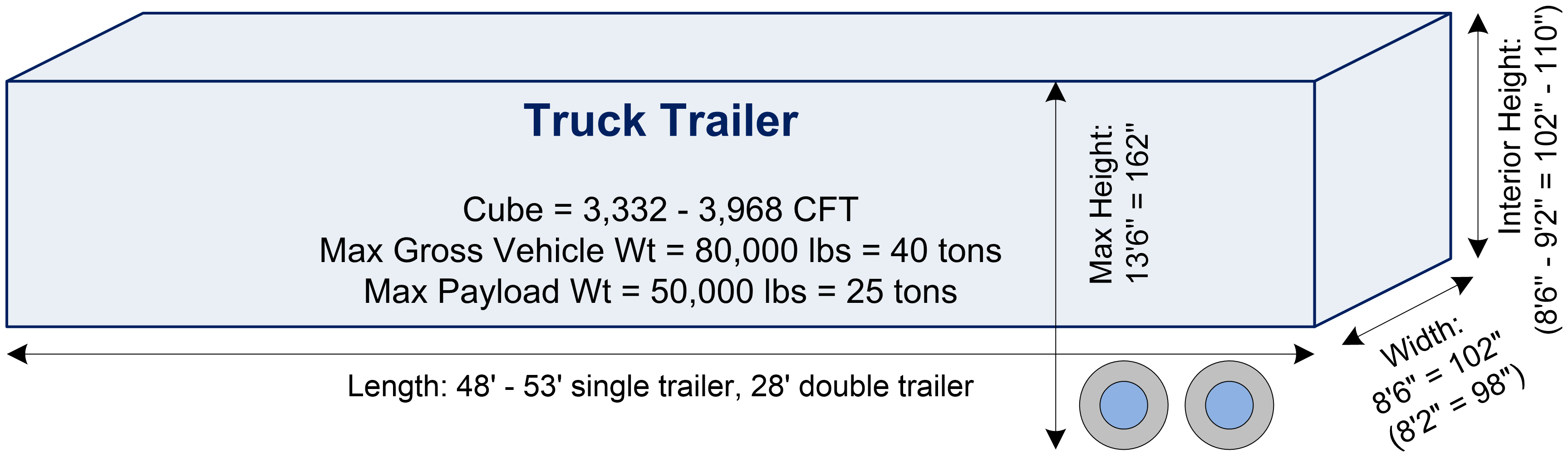
Figure 6: Why revenue per LOADED mile exceeds cost per mile. Every truck movement is red: solid where the trailer is loaded (L), dashed where it is empty (U). Only the Raleigh-to-Gainesville leg is paid for by this shipment, and the two repositioning legs either side of it are the carrier’s to absorb. The black line is the 532 miles between the two, which is a distance rather than a movement. Deadhead runs about 15% of all truck miles.

The three figures that turn the carrier’s cost into the shipper’s rate are its deadhead share, its cost per mile, and its margin:

15\%

= average deadhead travel, the share of total truck miles run empty

\$1.60

= cost per mile in 2004, loaded or not

\dfrac{\$1.60}{1 - 0.15}

= \$1.88, cost per loaded-mile

6.35\%

= average operating margin for trucking⁶

\dfrac{\$1.88}{1 - 0.0635}

\approx \$2.00, revenue per loaded-mile.

So $1.60 is the real number, and $2.00 is what it becomes once the empty miles and the margin – the carrier’s profit as a share of revenue – are added back. Deadhead has come down a little as carriers have grown better at matching loads, but 15% is stable enough to plan with.

NoteWhere the $1.60 per mile comes from

# Code block 1: the bottom-up TL cost per mile in 2004
defl = 100/132                     # PPI TL 2004 / PPI TL 2018

prime, over, infl = 0.0475, 0.0200, 0.0270
nom = prime + over                 # nominal interest rate
i   = nom - infl                   # real rate, the cost of capital

N     = 754_000/103_945            # avg mi to replacement / mi per yr
IV    = 175_000*defl               # new tractor-trailer, deflated to 2004
svpct = 0.20
SV    = svpct*IV
IVeff = IV - SV*(1 + i)^(-N)
K     = IVeff * (i / (1 - (1 + i)^(-N)))

mi   = 103_945                     # mi/yr
mpg  = 4.5                         # mi/gal
gal  = 1.78                        # $/gal
fpm  = gal/mpg                     # $/mi
fuel = fpm * mi                    # $/yr
tri  = 0.34 * 2.18 * mi * defl     # $0.34/mi in 1988, up then back
wage = defl * 45_330/(1 - 0.30)    # mean wage, grossed up for benefits
OC   = fuel + tri + wage
cpm  = (OC + K)/mi                 # $/mi, what the table reports

pct(x) = @sprintf("%.2f%%", 100x)
amt(x) = commafmt(round(Int, x))
num(x, d) = @sprintf("%.*f", d, x)

rows = [("**Interest rate**", "", ""),
        ("Prime rate[^cost-prime]", "", pct(prime)),
        ("Increase over prime", "", pct(over)),
        ("Nominal interest rate", "", pct(nom)),
        ("Current inflation rate[^cost-infl]", "", pct(infl)),
        ("Real interest rate", raw"$i$", pct(i)),
        ("**Lease**", "", ""),
        ("Economic life (yr)[^cost-life]", raw"$N$", num(N, 2)),
        (raw"Investment cost (\$)[^cost-iv]", raw"$IV$", amt(IV)),
        ("Salvage percentage", "", pct(svpct)),
        (raw"Salvage value (\$)", raw"$SV$", amt(SV)),
        (raw"Effective investment cost (\$)",
         raw"$IV^{\text{eff}}$", amt(IVeff)),
        (raw"Capital recovery cost (\$/yr)", raw"$K$", amt(K)),
        ("**Costing**", "", ""),
        ("Annual mileage (mi)[^cost-miles]", raw"$q$", amt(mi)),
        ("Fuel efficiency (mi/gal)[^cost-tsw]", "", num(mpg, 1)),
        (raw"Fuel cost per gallon (\$/gal)[^cost-eia]", "", num(gal, 3)),
        (raw"Fuel cost (\$/mi)", "", num(fpm, 4)),
        (raw"Annual fuel cost (\$/yr)", "", amt(fuel)),
        (raw"Tire, repair, insurance (\$/yr)[^cost-tri]", "", amt(tri)),
        (raw"Driver salary with benefits (\$/yr)[^cost-oes]",
         "", amt(wage)),
        (raw"Operating cost (\$/yr)", raw"$OC$", amt(OC)),
        (raw"Operating cost per mile (\$/mi)", "", num(OC/mi, 2)),
        (raw"Annual investment cost (\$/yr)", "", amt(K)),
        (raw"Investment cost per mile (\$/mi)", "", num(K/mi, 2)),
        (raw"**Total annual cost (\$/yr)**", "",
         "**" * amt(OC + K) * "**"),
        (raw"**Cost per mile (\$/mi)**", raw"$AC$",
         "**" * num(cpm, 2) * "**")]

# A group heading sits flush left; everything under it is indented one
# step, which is the shape the spreadsheet has and what makes a
# 27-row table readable as three blocks rather than as one long list.
label(a) = startswith(a, "**") ? "[" * a * "]{.tgroup}" :
                                 "[" * a * "]{.tindent}"

println("| Item | | 2004 |")
println("|:--|:--:|--:|")
for (a, b, c) in rows
    println("| ", label(a), " | ", b, " | ", c, " |")
end
println("\n: The bottom-up estimate of TL cost per mile in 2004. ",
        "{#tbl-tl-cost-2004 .fit}\n")

Table 4: The bottom-up estimate of TL cost per mile in 2004.

Item		2004
Interest rate
Prime rate7		4.75%
Increase over prime		2.00%
Nominal interest rate		6.75%
Current inflation rate8		2.70%
Real interest rate	i	4.05%
Lease
Economic life (yr)9	N	7.25
Investment cost ($)10	IV	132,576
Salvage percentage		20.00%
Salvage value ($)	SV	26,515
Effective investment cost ($)	IV^{\text{eff}}	112,695
Capital recovery cost ($/yr)	K	18,240
Costing
Annual mileage (mi)11	q	103,945
Fuel efficiency (mi/gal)12		4.5
Fuel cost per gallon ($/gal)13		1.780
Fuel cost ($/mi)		0.3956
Annual fuel cost ($/yr)		41,116
Tire, repair, insurance ($/yr)14		58,367
Driver salary with benefits ($/yr)15		49,058
Operating cost ($/yr)	OC	148,541
Operating cost per mile ($/mi)		1.43
Annual investment cost ($/yr)		18,240
Investment cost per mile ($/mi)		0.18
Total annual cost ($/yr)		166,781
Cost per mile ($/mi)	AC	1.60

The $1.60 is not an observed price, and Table 4 is where it comes from. It is built from a lease and an operating cost: a tractor-trailer with an economic life of 7.25 years and an effective investment cost of $112,695 recovers $18,240 a year in capital, and over 103,945 annual miles the operating cost, fuel at 4.5 mi/gal, tires, repair, insurance, and a driver salary of $49,058, comes to $148,541 a year. Together that is $166,781 a year, which over those miles is the $1.60.

Where the capital recovery cost comes from. The lease line is the one part of the table that is not simply a price looked up somewhere. A truck is bought once and used for years, while fuel and wages are paid continuously, and the two cannot be added until they are put on the same footing. Capital recovery cost does that: it is the equivalent uniform annual amount that a one-time investment and its eventual salvage value come to, at an interest rate that is the cost of capital.

\hphantom{\underset{\displaystyle AC}{\underset{\displaystyle K}{IV^{\text{eff}}}}}\mathllap{IV^{\text{eff}}} = \mathrlap{IV - SV\,(1 + i)^{-N}}\hphantom{\underset{\displaystyle \frac{K + OC}{q}}{\underset{\displaystyle IV^{\text{eff}} \left[ \frac{i}{1 - (1 + i)^{-N}} \right] = (IV - SV) \left[ \frac{i}{1 - (1 + i)^{-N}} \right] + SV \cdot i}{IV - SV\,(1 + i)^{-N}}}} \tag{4}

\hphantom{\underset{\displaystyle AC}{\underset{\displaystyle K}{IV^{\text{eff}}}}}\mathllap{K} = \mathrlap{IV^{\text{eff}} \left[ \frac{i}{1 - (1 + i)^{-N}} \right] = (IV - SV) \left[ \frac{i}{1 - (1 + i)^{-N}} \right] + SV \cdot i}\hphantom{\underset{\displaystyle \frac{K + OC}{q}}{\underset{\displaystyle IV^{\text{eff}} \left[ \frac{i}{1 - (1 + i)^{-N}} \right] = (IV - SV) \left[ \frac{i}{1 - (1 + i)^{-N}} \right] + SV \cdot i}{IV - SV\,(1 + i)^{-N}}}} \tag{5}

\hphantom{\underset{\displaystyle AC}{\underset{\displaystyle K}{IV^{\text{eff}}}}}\mathllap{AC} = \mathrlap{\frac{K + OC}{q}}\hphantom{\underset{\displaystyle \frac{K + OC}{q}}{\underset{\displaystyle IV^{\text{eff}} \left[ \frac{i}{1 - (1 + i)^{-N}} \right] = (IV - SV) \left[ \frac{i}{1 - (1 + i)^{-N}} \right] + SV \cdot i}{IV - SV\,(1 + i)^{-N}}}} \tag{6}

where

IV

= initial one-time investment cost ($)

SV

= one-time salvage value at time N ($)

OC

= operating cost per period ($/period)

i

= interest rate, the cost of capital (dimensionless)

q

= units per period, here miles per year (mi).

A lease is the cleanest way to see what K is: a lease payment is the capital recovery cost, because the vehicle goes back at the end. A loan payment is not, because the borrower still owns the vehicle when the loan is done.

Note: the average cost is not the present worth spread over the life. It is tempting to write AC = \left(IV^{\text{eff}} + PV \text{ of } OC\right) / (Nq), taking the present worth of everything and dividing by the total output. That is not Eq. 6 and it does not give the same answer: dividing a present worth by N spreads it evenly in nominal terms and so ignores the discounting that produced it. The capital recovery factor in Eq. 5 is what converts a present worth into a per-period amount correctly.

Every row of Table 4 follows from those three and a handful of published inputs, and the code that produced it folds under the table itself. Each input that was looked up rather than derived carries its source in the table.

Two of those inputs are worth pausing on, because they are where the estimate could most easily have gone wrong. The deflator is the same producer price index Sec. 2.8 is about, used in reverse: the vehicle cost and the wage are current figures brought back to 2004 so that every row sits in the same year’s dollars. And the driver wage is divided by 1 - 0.30 rather than multiplied by 1.30, because benefits are stated as a share of total compensation rather than as a markup on the wage.

The same three formulas size anything bought once and used over time. Run on a $32,000 car over five years at 12,000 miles a year, they give about 74 cents a mile, which is close to the Internal Revenue Service’s own standard mileage rate and a long way above what most drivers believe a mile costs them.

Adjusting to a later year. The 2004 estimate is carried forward by the ratio of the Producer Price Index for TL service to its 2004 value of 102.7:

r_{TL} = \frac{PPI_{TL}}{PPI_{TL}^{2004}} \times r_{2004} = \frac{PPI_{TL}}{102.7} \times \$2.00/\text{mi} \tag{7}

where

r_{TL}

= TL revenue per loaded truck-mile in the current period ($/mi)

PPI_{TL}

= Producer Price Index for TL service in that period (dimensionless).

Sec. 3.2 is where this is applied.

2.8 Producer Price Index

The two series that carry design constant 7 forward are published monthly by the Bureau of Labor Statistics.¹⁶

Where the data is and how to get it. Each series has a page of its own, and the series identifier is what addresses it: PCU484121484121 for truckload and PCU484122484122 for less-than-truckload. Going to data.bls.gov/timeseries/PCU484121484121 returns the whole monthly history, which is the fastest way to look at one value.

Table 5 and Table 6 are those two series from the base month, December 2003, to the present, laid out the way BLS lays them out so that the page and this lecture are recognizably the same table. Both are built from the committed data at render rather than copied from the website as an image, so they carry whatever the last refresh of data/ppi-trucking.csv returned. The years 2007 to 2015 are left out to hold each table to one screen, and the rightmost column is BLS’s own annual average rather than a mean taken here. Two markings carry over from BLS: the (P) on a value that is still provisional and will be revised, and the base date, which is December 2003 = 100.¹⁷ Three entries are set in bold, and each is a number the arithmetic below stands on: the base month itself, where the index is 100 by construction; the 2004 annual average, 102.7 for TL and 104.2 for LTL, the two divisors that carry a 2004 estimate forward; and the January 2018 reading this lecture is anchored at, chosen so that its arithmetic does not change from one year to the next.

Table 5: PCU484121484121 – PPI industry data for General freight trucking, long-distance TL, not seasonally adjusted. Base date 200312. Avg is the BLS annual average. A P marks a provisional value.

Year	Jan	Feb	Mar	Apr	May	Jun	Jul	Aug	Sep	Oct	Nov	Dec	Avg
2003												100.0
2004	100.3	101.1	101.2	101.5	101.9	102.5	102.6	103.0	104.0	104.7	105.4	104.8	102.7
2005	105.5	106.2	106.9	107.5	108.3	108.4	108.3	108.6	110.0	111.3	111.9	111.0	108.6
2006	110.3	110.4	110.4	110.8	112.1	112.4	112.5	113.2	113.4	113.0	112.5	112.3	112.0
⋮
2016	124.6	123.4	123.2	123.6	122.8	122.7	123.0	123.0	123.3	124.1	124.1	124.2	123.5
2017	124.4	124.7	124.2	124.3	124.0	124.2	124.2	125.9	126.6	126.6	128.5	130.3	125.6
2018	131.0	132.0	132.0	132.3	133.6	135.4	136.8	137.5	138.6	139.8	140.3	140.4	135.8
2019	139.9	138.6	138.2	136.7	137.3	137.7	136.8	136.1	136.6	136.6	140.1	141.0	138.0
2020	136.3	136.1	134.3	131.8	128.2	132.0	134.0	135.6	139.0	142.2	146.6	147.6	137.0
2021	146.1	151.3	154.7	159.3	162.1	159.3	159.9	164.7	169.6	173.8	182.6	187.7	164.3
2022	198.3	208.0	211.1	209.8	210.7	203.3	204.0	200.1	197.5	197.5	195.9	200.8	203.1
2023	187.2	194.5	202.3	184.4	192.6	190.5	178.7	173.3	182.0	184.0	187.2	177.7	186.2
2024	178.9	178.3	172.8	173.0	181.6	182.7	190.1	176.7	172.2	165.9	160.3	171.7	175.4
2025	181.7	179.4	165.8	175.1	178.5	168.4	180.9	182.3	186.1	184.9	189.1	181.1	179.4
2026	181.4	183.3	191.3	201.0	203.5P	198.8P	203.8P	207.6P

Table 6: PCU484122484122 – PPI industry data for General freight trucking, long-distance LTL, not seasonally adjusted. Base date 200312. Avg is the BLS annual average. A P marks a provisional value.

Year	Jan	Feb	Mar	Apr	May	Jun	Jul	Aug	Sep	Oct	Nov	Dec	Avg
2003												100.0
2004	101.1	101.5	101.9	101.4	102.2	103.4	104.8	105.1	106.3	107.1	108.1	108.0	104.2
2005	108.1	107.5	108.6	109.3	110.5	111.8	113.3	113.2	114.6	116.1	115.3	113.7	111.8
2006	114.7	114.3	115.4	116.6	119.2	119.2	119.5	120.3	119.7	117.5	117.6	117.9	117.7
⋮
2016	156.1	158.7	158.3	160.3	160.2	160.7	161.2	161.1	159.5	163.1	164.3	165.6	160.8
2017	166.4	166.8	166.7	167.0	168.0	167.9	169.7	169.9	173.3	173.5	175.1	175.5	170.0
2018	177.4	178.5	178.4	178.9	181.0	183.1	183.2	183.3	184.0	185.3	184.8	183.9	181.8
2019	188.5	188.8	187.8	186.2	189.9	190.3	188.1	190.1	187.8	188.7	189.3	185.2	188.4
2020	193.6	191.1	189.7	188.4	187.7	186.1	190.3	189.9	185.5	189.6	187.7	187.1	188.9
2021	196.7	196.8	202.5	203.4	203.7	210.7	208.3	207.8	209.3	211.7	218.0	218.1	207.3
2022	222.9	220.7	239.5	243.6	251.9	258.8	248.6	242.1	242.9	237.3	242.4	233.6	240.4
2023	240.5	236.3	233.3	228.2	231.5	230.7	230.8	240.8	242.9	244.3	240.9	236.2	236.4
2024	242.2	244.2	245.5	246.9	244.8	241.7	247.5	243.8	243.0	243.3	243.4	243.4	244.2
2025	257.4	259.2	259.0	259.1	258.1	261.0	265.4	268.4	267.0	266.3	268.2	267.3	263.0
2026	270.6	272.9	277.7	311.0	312.1P	308.0P	293.7P	306.8P

One property of the index is worth knowing before any figure is quoted from it. A recently published value is provisional and is revised later. January 2018 was first published as 131.4 for TL and 179.4 for LTL; the revised values are 131.0 and 177.4. This lecture uses the revised values throughout.

3. Truckload shipments

Everything so far has been about what a shipper can buy and what the standing numbers are. From here the lecture follows one shipment through every charge it can be assessed, and the shipment is the same one Lecture 3.3 continues with.

Example 1: Truck shipment from Raleigh to Gainesville

A product is shipped in cartons from Raleigh, NC (27606) to Gainesville, FL (32606). Each identical carton weighs 40 lb and occupies 9 ft³ (its cube). The linear dimensions of each unit are not known for TL and LTL, and the cartons can be stacked on top of each other in a trailer. Additional information and data is presented only when it is needed to determine an answer.

3.1 Maximum payload

A trailer is constrained by weight and by cubic volume at the same time, and which one binds is decided by the density of the load alone. The maximum payload is the maximum size of each truckload:

q_{\max} = \min\left\{ q_{\max}^{wt},\, q_{\max}^{cu} \right\} = \min\left\{ K_{wt},\, \frac{s K_{cu}}{2000} \right\} \tag{8}

where

q_{\max}

= maximum payload (ton)

s

= item density (lb/ft³)

K_{wt}

= weight capacity of truck trailer (ton)

K_{cu}

= cube capacity of truck trailer (ft³).

The cube term is obtained by solving for q in K_{cu} = q / (s/2000), where s/2000 is the density in ton/ft³.

Example 1(a): Maximum payload

Assuming that the product is to be shipped P2P TL, determine the maximum payload for each trailer used for the shipment.

# Code block 2: density and maximum payload
uwt = 40                           # lb/unit
ucu = 9                            # ft^3/unit
@show s = uwt/ucu                  # lb/ft^3
Kwt = 25                           # ton
Kcu = 2750                         # ft^3
@show qmax = min(Kwt, s*Kcu/2000)  # ton
# = maxpayld(s; Kwt=Kwt, Kcu=Kcu)

s = uwt / ucu = 4.444444444444445
qmax = min(Kwt, (s * Kcu) / 2000) = 6.111111111111112

6.111111111111112

q_{\max} is well under the 25-ton weight cap, so this load cubes out: the trailer fills before it gets heavy.

q_{\max} = 6.1111 ton, set by cube rather than by weight.

3.2 Transport charge and PPI

The TL transport charge assumes that any portion of the load exceeding the maximum payload is still transported TL using additional trucks:

c_{TL} = \left\lceil \frac{q}{q_{\max}} \right\rceil r_{TL}\, d \tag{9}

where

c_{TL}

= TL transport charge ($)

q

= shipment weight (ton)

d

= road distance between the O-D pair (mi).

In determining the TL transport charge, revenue per loaded-truck-mile is used instead of the cost per truck-mile because the user of the rate model is assumed to be a shipper (i.e., customer) buying TL service from a carrier on the basis of dollars-per-loaded-mile.

Example 1(b): Number of truckloads

On Jan 10, 2018, 300 cartons of the product were shipped. Determine how many truckloads were required for this shipment.

# Code block 3: shipment size and truckload count
udTL = 300                       # cartons
@show qTL = udTL*(uwt/2000)      # ton
@show nTL = ceil(Int, qTL/qmax)  # truckloads

qTL = udTL * (uwt / 2000) = 6.0
nTL = ceil(Int, qTL / qmax) = 1

1

q = 6.0 ton, requiring 1 truckload.

Example 1(c): Estimated TL transport charge

Before contacting the carrier to negotiate, and using the January 2018 PPI, determine the estimated TL transport charge for this shipment.

# Code block 4: the TL rate and charge at the Jan 2018 index
d = 532                               # mi, Google Maps road distance
ppiTL = 131.0                         # TL PPI for Jan 2018
@show rTL = 2.00ppiTL/102.7           # $/mi
@show cTL = charge_tl(qTL, s, d; r = rTL, Kwt = Kwt,
                      Kcu = Kcu, ppi = ppiTL)  # $

rTL = (2.0ppiTL) / 102.7 = 2.5511197663096397
cTL = charge_tl(qTL, s, d; r = rTL, Kwt = Kwt, Kcu = Kcu, ppi = ppiTL) = 1357.1957156767282

1357.1957156767282

r_{TL} = $2.55/mi, so c_{TL} = $1357.2.

3.3 Aggregate shipment

When multiple items are shipped together as part of a single load, then it is convenient to view them as a single demand-weighted aggregate shipment, where, for m items, the aggregate weight and aggregate density are

q_\text{agg} = \sum_{i=1}^{m} q_i , \qquad s_\text{agg} = \frac{q_\text{agg}}{\sum_{i=1}^{m} q_i / s_i} \tag{10}

where

q_i

= weight of item i (ton)

s_i

= density of item i (lb/ft³).

The aggregate density is a weighted harmonic mean rather than an arithmetic one, because what adds across items is volume, not density. Logjam’s aggshmt performs the same reduction over a DataFrame of shipments, and Lecture 3.3 uses it once demand rates replace shipment sizes.

4. Less-than-truckload shipments

LTL is rated differently from TL, and the difference is not merely a smaller number. A TL charge is a rate per mile multiplied by a distance, with the load entering only through the number of trucks. An LTL charge depends on the weight and the density of the load as well as the distance, because the carrier handles the freight at every terminal it passes through.

4.1 Rate estimate

In most commercial transportation management and planning systems, LTL rates are determined using tariff tables (e.g., CzarLite), but this requires the shipper/decision maker to purchase access to the tariff tables and, further, to know what discount to apply to the tariff rates. The following model was developed from tariff rate tables and provides a general means of estimating rates for LTL transport between origin-destination (O-D) pairs located anywhere within the continental United States.¹⁸ Since it requires only distance, weight, and density as inputs and allows direct comparison of LTL and TL rates, it can be used in the earliest stages of logistics network design. The LTL transport charge, c_{LTL}, is the estimated rate over the size and the distance of the shipment, and the rate is what the model supplies:

\hphantom{\underset{\displaystyle r_{LTL}}{c_{LTL}}}\mathllap{c_{LTL}} = \mathrlap{r_{LTL}\, q\, d}\hphantom{\underset{\displaystyle PPI_{LTL} \left[ \frac{\frac{s^2}{8} + 14} {\left( q^{1/7} d^{15/29} - \frac{7}{2} \right)\left( s^2 + 2 s + 14 \right)} \right]}{r_{LTL}\, q\, d}} \tag{11}

\hphantom{\underset{\displaystyle r_{LTL}}{c_{LTL}}}\mathllap{r_{LTL}} = \mathrlap{PPI_{LTL} \left[ \frac{\frac{s^2}{8} + 14} {\left( q^{1/7} d^{15/29} - \frac{7}{2} \right)\left( s^2 + 2 s + 14 \right)} \right]}\hphantom{\underset{\displaystyle PPI_{LTL} \left[ \frac{\frac{s^2}{8} + 14} {\left( q^{1/7} d^{15/29} - \frac{7}{2} \right)\left( s^2 + 2 s + 14 \right)} \right]}{r_{LTL}\, q\, d}} \tag{12}

where

r_{LTL}

= estimated LTL rate ($/ton-mi)

PPI_{LTL}

= Producer Price Index for LTL service (104.2 in 2004).

The model reflects average industry rates and allows rate estimates to be adjusted to current economic conditions by using the current Producer Price Index for LTL service. Note that, in actuality, an LTL shipment between any origin and destination is likely to travel a longer distance than the road distance d because it will travel through one or more transshipment terminals along its journey. However, the road distance between O-D pairs is the only readily available measure of distance, and, since the particular network of transshipment terminals is specific to each LTL carrier, it is the only reasonable measure. The model is independent of the particular characteristics of any O-D pair and, since the only parameter that distinguishes O-D pairs is road distance, the resulting rate estimate is symmetric with respect to O-D order, with such differences being treated as noise.

The range the estimate is valid over is part of the estimate. Eq. 12 holds for 37 \le d \le 3{,}354 mi, 0.075 \le q \le 5 ton, and 2000\,q/s \le 650 ft³. These conditions represent the range of input data that produced the estimate, and they also ensure that the denominator stays positive. Outside them the formula does not fail, it returns a negative rate: pushing q and d low enough drives q^{1/7} d^{15/29} - 7/2 below zero, and the result is a confident, wrong, negative charge. K_{wt} and K_{cu}, meanwhile, do not appear anywhere in Eq. 12, and that is not an oversight. The trailer’s capacities are a truckload constraint: they decide how much fits on a truck the shipper is paying for whole. An LTL shipment rides with other freight, so the carrier’s trailer capacity is the carrier’s problem and never enters the rate.

NoteHow the formula was fitted

Eq. 12 is Kay and Warsing’s top-down regression onto published tariff rates rather than a model of a carrier’s costs.¹⁹ One can verify by inspection that actual tariff-based LTL rates are inversely proportional to the density, weight, and distance of the shipment, and that observation is the basis for the specification of the initial model:

r_{LTL}^{(1)}(q, s, d) = \frac{\beta_1}{\beta_2 + q^{\beta_3} s^{\beta_4} d^{\beta_5}}

That form frames the relationship in its most general form, allowing the parameters to be tested empirically from a given set of data containing LTL rates and their corresponding shipment weights, shipment distances, and shipment densities.

The regression method involves minimizing the weighted absolute relative error between the estimated rate for a given weight-density-distance triple, r_{LTL}(q, s, d), and the raw (undiscounted) CzarLite tariff rate (SMC3 2005) for those same q, s, and d values, r_\text{tariff}(q, s, d):

\min \sum_{q \in Q} \sum_{s \in S} \sum_{d \in D} w_q w_s w_d \left| \frac{r_{LTL}(q, s, d)}{r_\text{tariff}(q, s, d)} - 1 \right|

where w_q, w_s, and w_d are weighting factors and Q, S, and D are the sets of shipment weights, densities, and distances, respectively, from which to draw the values of the independent variables for the regression. The weighting factors represent the relative likelihoods of various shipment parameter values. Since shipment weight and density are not independent in practice, w_q and w_s are replaced with a combined factor w_{sq} that reflects this dependence.

Getting from that general form to the one the lecture uses took seven steps. A total of six regression steps were performed, using as many as 10 out of the 11 parameters in the full model to estimate the LTL rate.

Table 7: The analysis steps and the weighted absolute relative error at each.

Step	1 Initial	2 Residual fit	3 Full	4 Simplify	5 Normalize	6 Simplify	7 Round
WARE	20.49%	—	11.37%	11.66%	11.66%	11.66%	11.93%

As parameters were dropped from the model in simplifying it (Steps 3 to 4), some of the remaining parameters changed rather dramatically. Steps 4 to 5 represent only a scaling step, which altered only certain coefficient and constant terms, with the remaining steps representing the final tuning of the parameters. Table 7 is also what the readable form cost: rounding the exponents to the fractions Eq. 12 carries gives up about a quarter of a percentage point of accuracy.

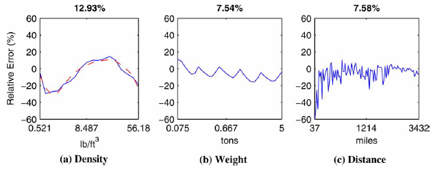
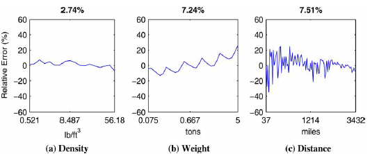
Figure 7: Relative error against density, weight and distance, for the initial model (top) and the full model (bottom).²⁰

Fig. 7 is where the improvement went. The density panel falls from 12.93% to 2.74%, which is the term in s doing its work; weight and distance barely move, at 7.54% to 7.24% and 7.58% to 7.51%.

Example 1(d): Estimated LTL transport charge

Using the January 2018 PPI LTL rate estimate, determine the transport charge to ship 15 cartons LTL.

# Code block 5: the LTL rate estimate and charge
udLTL = 15                                # cartons
@show qLTL = udLTL*(uwt/2000)             # ton
ppiLTL = 177.4                            # LTL PPI for Jan 2018

@show rLTL = rate_ltl(qLTL, s, d; ppi = ppiLTL)    # $/ton-mi
@show cLTL = charge_ltl(qLTL, s, d; ppi = ppiLTL)  # $

qLTL = udLTL * (uwt / 2000) = 0.3
rLTL = rate_ltl(qLTL, s, d; ppi = ppiLTL) = 3.7770239841173217
cLTL = charge_ltl(qLTL, s, d; ppi = ppiLTL) = 602.8130278651246

602.8130278651246

r_{LTL} = $3.78/ton-mi, so c_{LTL} = $602.81.

4.2 Comparing TL and LTL

At 0.3 ton, LTL is much the cheaper service. At 6 tons, TL is. Somewhere between them the two charges are equal, and that crossing is what decides which service a given shipment should use.

Example 1(e): The shipment size at which the charges are equal

Determine the shipment size at which the TL and LTL charges are equal.

The two charges as functions of q are c_{TL}(q) from Eq. 9 and c_{LTL}(q) = r_{LTL}(q)\,q\,d from Eq. 12. Their crossing is the q at which the absolute difference is zero, which is a univariate minimization:

q_I = \arg\min_q \left| c_{TL}(q) - c_{LTL}(q) \right| \tag{13}

# Code block 6: the TL/LTL break-even shipment size
cTLh(q)  = charge_tl(q, s, d; r = rTL, Kwt = Kwt,
                     Kcu = Kcu, ppi = ppiTL)
cLTLh(q) = charge_ltl(q, s, d; ppi = ppiLTL)

# The search stops at the rate estimate's own upper bound rather
# than at qmax. Sec. 4.1 gives it as 2000q/s <= 650 ft^3, which for
# this load is 1.44 ton, and `rate_ltl` returns Inf above it rather
# than extrapolating -- so a search over the whole trailer would be
# optimising a constant.
qLTLmax = 650s/2000
gap(q) = abs(cTLh(q) - cLTLh(q))     # zero where the two are equal
@show qI = optimize(gap, 0.075, qLTLmax).minimizer
@show cTLh(qI), cLTLh(qI)  # equal at the crossing

qI = (optimize(gap, 0.075, qLTLmax)).minimizer = 0.7959529639553807
(cTLh(qI), cLTLh(qI)) = (1357.1957156767282, 1357.1957214745564)

(1357.1957156767282, 1357.1957214745564)

# `charge_tl` and `charge_ltl` ALREADY floor at their minimum
# charges, which are Sec. 4.3's subject, so the independent charge
# is the smaller of the two rather than the smaller of two maxima.
c0h(q) = min(cTLh(q), cLTLh(q))

# From ONE POUND rather than from zero, which is what the example
# asks for. At exactly zero `ceil(0/qmax)` is zero trucks, so the
# TL charge is zero and the curve would drop to the axis; a pound
# in, the left end is the LTL minimum charge.
qs = range(1/2000, 2qI; length = 1200)
fig = Figure(size = (687, 400))
ax = Axis(fig[1, 1];
          xlabel = "Shipment size (ton)",
          ylabel = "Transport charge (\$)",
          title = "Indifference point between TL and LTL",
          titlesize = 17, xlabelsize = 16, ylabelsize = 16,
          xticklabelsize = 14, yticklabelsize = 14)
lines!(ax, qs, c0h.(qs);
       color = RGBf(0.13, 0.35, 0.60), linewidth = 2.2)
# An OPEN circle, as the MATLAB draws it: `plot(qI, c0h(qI), 'ro')`.
# A filled marker of the same colour as the curve is what made the
# point hard to see.
scatter!(ax, [qI], [cTLh(qI)]; color = :white,
         markersize = 13, strokewidth = 2.2,
         strokecolor = RGBf(0.78, 0.16, 0.18))
text!(ax, qI, cTLh(qI); text = "  qI = $(round(qI, digits=4)) ton",
      align = (:left, :top), fontsize = 14,
      color = RGBf(0.78, 0.16, 0.18))
# Both axes start AT zero, so the origin sits in the corner.
# Makie pads by default, which lifts the zero off it and makes
# the two axes look as though they do not meet.
xlims!(ax, 0, 2qI)
# The top is a round number so the tick set lands INSIDE the
# limits and the zero is drawn: with a ragged top Makie drops
# the end ticks, and the one it dropped was the y-axis zero.
ylims!(ax, 0, 1500)
# The zero sits on the corner, as it does on the slide.
ax.xticks = 0:0.5:1.5
ax.yticks = 0:500:1500
fig

Figure 8: The independent charge over the range where the two services cross. LTL governs to the left of the marked point and a single truckload to the right, where the charge stops depending on how much of the trailer is used.

Fig. 8 is the same charge drawn over the range where the change happens.

q_I = 0.796 ton. Below it LTL is cheaper; above it a full truckload is.

That answers a question a shipper asks the other way round too. A load just over one truckload can go as two full truckloads, or as one truckload plus the remainder sent LTL, and splitting costs more for any remainder above 0.796 ton, because LTL is expensive per ton even in small quantities.

# Class and average density, read off the class-density table.
classes = [("Class 300", 2.49), ("Class 100", 9.72),
           ("Class 85", 12.72), ("Class 60", 32.16)]
# The estimate's upper bound is the SMALLER of its weight bound
# and its cube bound, and for a light class the cube one binds
# first: Class 300 stops at 0.81 ton, not at 5.
qtop(sk) = min(5.0, 650sk/2000)

fig = Figure(size = (687, 520))
for (k, (nm, sk)) in enumerate(classes)
    row, col = fldmod1(k, 2)
    ax = Axis(fig[row, col];
              xlabel = "Shipment size (ton)",
              ylabel = "Rate (\$/ton-mi)",
              title = "$nm  ($sk lb/ft³)",
              titlesize = 15, xlabelsize = 14, ylabelsize = 14,
              xticklabelsize = 13, yticklabelsize = 13)
    qmk = min(Kwt, sk*Kcu/2000)          # this class's maximum payload
    rateTL(q)  = ceil(q/qmk) * rTL / q   # $/ton-mi, from the charge
    rateL(q)   = rate_ltl(q, sk, d; ppi = ppiLTL)

    qs = range(0.1, Kwt; length = 3000)
    lines!(ax, qs, rateTL.(qs); color = RGBf(0.13, 0.45, 0.25),
           linewidth = 2.0, label = "TL")
    ql = range(0.1, qtop(sk); length = 1200)
    lines!(ax, ql, rateL.(ql); color = RGBf(0.78, 0.16, 0.18),
           linewidth = 2.0, linestyle = :dashdot, label = "LTL")

    # The equal-rate size, found as qI was: a bounded 1-D search.
    qe = optimize(q -> abs(rateTL(q) - rateL(q)),
                  0.1, qtop(sk)).minimizer
    scatter!(ax, [qe], [rateL(qe)]; color = RGBf(0.20, 0.30, 0.75),
             markersize = 11)
    text!(ax, qe, rateL(qe); text = "  $(round(qe, digits = 1)) ton",
          align = (:left, :bottom), fontsize = 13,
          color = RGBf(0.20, 0.30, 0.75))
    xlims!(ax, 0, Kwt)
    # EACH PANEL GETS ITS OWN y LIMIT. The chapter fixes one scale
    # across all four because its rates are on the 2004 index; on
    # this lecture's January-2018 index the LTL rate for Class 300
    # runs clean off a shared scale and takes its crossing with it,
    # which is a panel that shows nothing.
    ylims!(ax, 0, 2.2 * rateL(qe))
    k == 1 && axislegend(ax; position = :rt, labelsize = 13)
end
fig

Figure 9: Rate per ton-mile against shipment size, for four freight classes on the same 532-mile lane. TL falls as the trailer fills and jumps each time another truck is needed; LTL falls smoothly. The marked point is the size at which the two are equal, and it moves right as the load gets denser. The LTL curve is drawn only over the range Eq. 12 is valid for.

Fig. 9 is Eq. 12 and the TL charge set against each other over four classes rather than one. The TL rate is a sawtooth because a truckload is bought whole: the rate per ton-mile falls as the trailer fills and jumps back up the moment a second truck is needed. The LTL rate falls smoothly, because nothing is bought whole. Where they cross is the size at which the two services cost the same, and it moves to the right as the load gets denser, from well under a ton for Class 300 to several tons for Class 60.

The arithmetic determines which service is cheaper, and it does not determine which service to use. Where the two charges are close, the full truckload is the better choice on grounds the charge does not capture. An LTL shipment typically takes longer, because it is handled at every terminal on its route. It is more likely to be damaged, for the same reason. And although a shipper carries insurance, reimbursement in practice only follows significant damage. So LTL is worth choosing when the saving is substantial, not when it is marginal.

NoteUnivariate optimization, and Brent’s method

Eq. 13 is solved numerically rather than in closed form, and the technique recurs throughout the course, so it is worth seeing once on its own.

A univariate optimization finds

x^* = \arg\min_x \left\{ f(x) : LB \le x \le UB \right\}, \qquad TC^* = f(x^*) \tag{14}

where

x^*

= minimizing value of the decision variable

LB

= lower bound on the search interval

UB

= upper bound on the search interval

f

= objective function.

Interval search. Divide the interval, evaluate f at interior points, and discard the portion that cannot contain the minimum. Dividing into thirds discards one third per iteration.

Golden section. Placing the two interior points at the golden ratio rather than at the thirds improves the reduction a little, from about 0.33 of the interval to 0.38. The better part is elsewhere. Interval search recomputes the objective at both interior points on every pass; golden section is arranged so that one of the two points, and its function value, carries over to the next iteration. It therefore costs one new evaluation per pass instead of two, which halves the number of evaluations. For an analytical function that is nothing, milliseconds of processor time. But the thing being evaluated might be a simulation that takes several minutes even on a fast computer, and halving the count is then what makes this the basis of industrial optimization rather than a curiosity.

Parabolic interpolation. Pick three points, a triplet, and fit the parabola through them. Three points give three equations in the three coefficients, so the fit is one linear solve rather than a search. A parabola’s minimum is then known analytically once those coefficients are in hand, so instead of shrinking an interval the method steps straight to it.

Brent’s method. Parabolic interpolation is not surefire, and how it fails is worth seeing. If the three points do not enclose the minimum, which is easy enough when the bounds were guessed rather than plotted, the fitted parabola has its own minimum nowhere near the function’s: a bad parabolic update. Brent’s method (1973) is the intelligent way of using parabolic interpolation when it can be trusted, and the test is whether the calculated minimum falls between the first and third points of the triplet. While it does, the method keeps interpolating; the moment it falls outside, the method switches to golden section, and switches back once interpolation is improving again. That is the go-to technique in Optim, in SciPy, in MATLAB and in essentially any scientific programming language, and it has been since 1973.

Finding a root or an intersection. A minimizer can find where a function is zero, and therefore where two functions cross, by minimizing a non-negative function that vanishes there. Minimizing |f(x)| or f(x)^2 drives f to zero, which is exactly what Eq. 13 does with the difference of the two charge functions. The bracket matters: a function with several roots has several minima, and the bounds decide which one is found.

# Code block 7: the three roots of f(x) = x - x^3, found by bracketing
f(x) = x - x^3
g(x) = f(x)^2                            # non-negative, zero at each root
@show optimize(g, -2.0, -0.5).minimizer  # near -1
@show optimize(g, -0.5,  0.5).minimizer  # near  0
@show optimize(g,  0.5,  2.0).minimizer  # near +1

(optimize(g, -2.0, -0.5)).minimizer = -0.9999999992556936
(optimize(g, -0.5, 0.5)).minimizer = -1.3877787807814457e-17
(optimize(g, 0.5, 2.0)).minimizer = 0.9999999992556936

0.9999999992556936

4.3 Minimum and independent charges

In practice, in addition to the basic P2P TL and LTL charges, there is a minimum charge associated with any shipment that corresponds to the cost of providing the transport service that is not related to the weight of the shipment. There is a separate estimated minimum charge for TL and LTL:

MC_{TL} = \left(\frac{r_{TL}}{2}\right) 45 , \qquad MC_{LTL} = \left(\frac{PPI_{LTL}}{104.2}\right) \left( 45 + \frac{d^{28/19}}{1625} \right) \tag{15}

where d > 0 and q > 0, and MC_{TL} = MC_{LTL} = 0 for d = 0 or q = 0.

The minimum charge for TL is independent of distance and depends solely on loading and unloading costs at the origin and destination of the shipment, while the charge for LTL is a function of the distance of the shipment because each shipment is loaded and unloaded at each LTL terminal visited in transit and the number of terminals visited increases with the length of the shipment.

Example 1(f): TL and LTL minimum charges

Determine the TL and LTL minimum charges, and account for why neither depends on the size of the shipment while only the LTL charge depends on its distance.

# Code block 8: the two minimum charges
@show MC_TL  = mincharge_tl(; ppi = ppiTL)      # $
@show MC_LTL = mincharge_ltl(d; ppi = ppiLTL)   # $

MC_TL = mincharge_tl(; ppi = ppiTL) = 57.40019474196689
MC_LTL = mincharge_ltl(d; ppi = ppiLTL) = 87.5107523114767

87.5107523114767

MC_{TL} = $57.4, MC_{LTL} = $87.51.

An independent shipment corresponds to either a P2P TL shipment or a LTL shipment. It represents an alternative to a multi-stop consolidated load, where multiple shipments are carried on a single truck at the same time. Using the TL and LTL transport and minimum charges,

c_0(q) = \min\Bigl\{ \max\bigl\{ c_{TL}(q),\, MC_{TL} \bigr\},\; \max\bigl\{ c_{LTL}(q),\, MC_{LTL} \bigr\} \Bigr\} \tag{16}

where

c_0

= independent transport charge ($).

Example 1(g): The independent transport charge

Determine the independent transport charge over the range of shipment sizes from one pound to one and a fifth truckloads, and identify the two points at which the governing term changes.

# The two charges already carry their minimum charges, so the
# independent charge is the smaller of them.
c0(q) = min(cTLh(q), cLTLh(q))

# From ONE POUND, which is what the statement asks for and what
# makes the flat left end the LTL minimum charge the result box
# prints. At exactly zero the TL charge is zero trucks.
qs = range(1/2000, 1.2qmax; length = 2400)

# A SPLIT HORIZONTAL AXIS, because on a linear one the whole LTL
# branch is the first 11% of the width and reads as a straight
# line. `u` gives the first ton half the axis and the remaining
# 6.3 tons the other half, so the break-even lands at 40% of the
# width with its curvature intact.
#
# LINEAR INSIDE EACH PIECE, which is the point. c_LTL grows about
# as q^0.85 and is concave; against sqrt(q) that becomes u^1.7 and
# reads as CONVEX. Every smooth transform that expands the low end
# is itself concave, so every one of them bends the curve the
# wrong way. A split scale preserves the shape it separates.
const QSPLIT = 1.0                      # ton, where the axis breaks
u(q) = q <= QSPLIT ? 0.5q/QSPLIT :
       0.5 + 0.5(q - QSPLIT)/(1.2qmax - QSPLIT)

fig = Figure(size = (687, 430))
ax = Axis(fig[1, 1];
          xlabel = "Shipment size (ton)",
          ylabel = "Transport charge (\$)",
          title = "Independent charge: Class 200, 27606 to 32606",
          titlesize = 17, xlabelsize = 16, ylabelsize = 16,
          xticklabelsize = 14, yticklabelsize = 14)
# The seam, drawn faintly so the change of scale is visible
# rather than something the reader has to infer from the ticks.
vlines!(ax, [0.5]; color = (:black, 0.28), linewidth = 1,
        linestyle = :dash)
lines!(ax, u.(qs), c0.(qs);
       color = RGBf(0.13, 0.35, 0.60), linewidth = 2.2)
# Open circles, the MATLAB's own markers: red at the break-even,
# cyan at one truckload.
scatter!(ax, [u(qI)], [c0(qI)]; color = :white, markersize = 13,
         strokewidth = 2.2, strokecolor = RGBf(0.78, 0.16, 0.18))
text!(ax, u(qI), c0(qI); text = "  qI = $(round(qI, digits=3)) ton",
      align = (:left, :bottom), fontsize = 14,
      color = RGBf(0.78, 0.16, 0.18))
scatter!(ax, [u(qmax)], [c0(qmax)]; color = :white, markersize = 13,
         strokewidth = 2.2, strokecolor = RGBf(0.10, 0.55, 0.65))
text!(ax, u(qmax), c0(qmax);
      text = "qmax = $(round(qmax, digits=3)) ton  ",
      align = (:right, :bottom), fontsize = 14,
      color = RGBf(0.10, 0.55, 0.65))
# Both axes start AT zero, so the origin sits in the corner. Makie pads by
# default, which lifts the zero off it (instructor, 2026-09-22).
xlims!(ax, 0, 1)
ylims!(ax, 0, 1.08 * c0(1.2qmax))
# A tick AT zero, so the zero is ON the corner rather than the
# first tick inboard of it: Makie picks its own round numbers
# and skips the endpoint.
# The ticks carry the REAL shipment sizes, placed where the
# split scale puts them, so the axis reads in tons throughout.
xt = [0, 0.25, 0.5, 0.75, 1, 2, 3, 4, 5, 6, 7]
lbl(x) = isinteger(x) ? string(Int(x)) : string(x)
ax.xticks = (u.(xt), lbl.(xt))
ax.yticks = 0:1000:3000
fig

Figure 10: The independent transport charge for a Class 200 shipment from 27606 to 32606. The LTL estimate governs below the break-even, a single truckload above it, and each is floored at its own minimum charge. The flat left end is the LTL minimum charge; the step at the maximum payload is the second truck. The horizontal axis is split at one ton, marked by the dashed rule, so that the LTL branch has room to show its shape.

Fig. 10 is that charge over the whole range, and the two points marked on it are the two the statement asks for.

The charge is floored at $87.51, follows the LTL estimate to 0.796 ton, and is a single truckload at $1357.2 from there to q_{\max}.

5. Freight class and LTL tariffs

The estimate of Sec. 4.1 is a regression over average industry rates. What a carrier actually quotes comes from a tariff, and a tariff prices a shipment by its freight class and its weight. This section reads a charge out of a real tariff for the same shipment, and then sets the two answers side by side.

5.1 Class and density

LTL rates are dependent on a number of factors, prominent among them being the specific origin and destination, the weight of the shipment, and the freight class to which the goods being shipped belong. The specific characteristics of each item that impact its transport cost need to be considered in assigning each item to be transported to a freight class, including the following considerations:

• Load density, e.g., a large item will cube-out a trailer sooner than a smaller item that has the same weight.
• Special handling, e.g., fragile loads; hazardous materials; unit load size, since it is more costly to handle several small loads that comprise a single shipment that together have the weight as a single large unit load.
• Stowability, e.g., some items can be nested.
• Liability, e.g., high value items are more expensive to insure while in transit.

The National Motor Freight Classification is typically used to determine the rating of an item.²¹ Most LTL carriers have a Freight All Kinds (FAK) rate that can be used for any item that cannot be classified. Discounts of up to 15% from the published rates are usually available for a single one-time shipment; when a firm has frequent shipments, discounts of 30–65% can usually be negotiated.

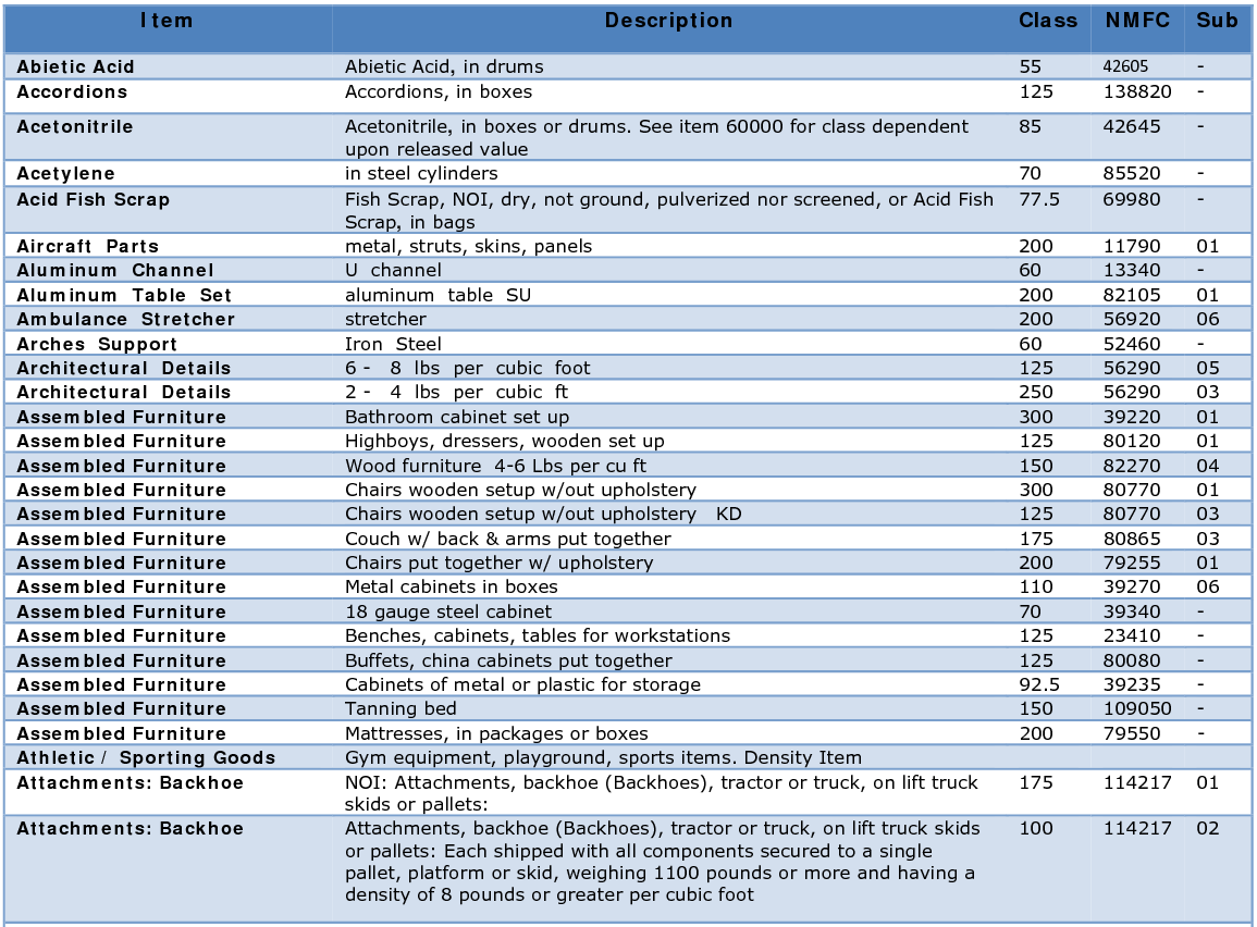
Figure 11: A page of the classification’s listings. Each row gives an item, a description precise enough to separate two forms of the same thing, and the class that follows from it.²²

Fig. 11 is what a classification actually looks like, and the second column is the part worth noticing: two entries for Assembled Furniture differ only in whether the chairs come with upholstery, and that difference is 125 against 300.

Table 8 shows the minimum density and average density for each freight class. Also shown is the maximum weight for a shipment assuming a maximum physical payload of 25 tons (50,000 lb) and the maximum cubic volume for a shipment assuming a maximum effective payload of 2,750 ft³.

Table 8: Class–density relationship. Italics indicate the value at capacity.

Class	Min density (lb/ft3)	Avg density (lb/ft3)	Max weight (ton)	Max cube (ft3)
500	—	0.52	0.72	2,750
400	1	1.49	2.06	2,750
300	2	2.49	3.43	2,750
250	3	3.49	4.80	2,750
200	4	4.49	6.17	2,750
175	5	5.49	7.55	2,750
150	6	6.49	8.92	2,750
125	7	7.49	10.30	2,750
110	8	8.49	11.67	2,750
100	9	9.72	13.37	2,750
92.5	10.5	11.22	15.43	2,750
85	12	12.72	17.49	2,750
77.5	13.5	14.22	19.55	2,750
70	15	18.01	24.76	2,750
65	22.5	25.50	25	1,961
60	30	32.16	25	1,555
55	35	39.68	25	1,260
50	50	56.18	25	890

The ideal density (18.18 lb/ft³) is the density at which a full truckload is simultaneously at the tractor-trailer’s cubic capacity and its weight capacity. An average freight mix at this density best utilizes both the weight and cube capacities of a tractor-trailer. Shipments weigh out when their average density is greater than the critical density and cube out when it is less. Note that Class 100 represents the “average” load and has an average density of 9.72 lb/ft³, which is in the range of densities that cube out a trailer.

NoteThe same threshold in the other two modes

Density decides which of a vehicle’s two capacities runs out first, and the threshold is not the same in every mode. Lecture 3.1 makes the point without figures because the trailer numbers had not been introduced; they have now.

Table 9: The density above which weight binds before cube, by mode.²³

Mode	Weighs out above
Ocean, 40-ft dry container	25 lb/ft3	394 kg/m3
Road, van semi-trailer	18.18 lb/ft3	291 kg/m3
Air	10.40 lb/ft3	167 kg/m3
Average load (Class 100)	9.72 lb/ft3	156 kg/m3

Table 9 sets the average load against each threshold. On the road it sits at 53% of it and cubes out with room to spare, which is why van semi-trailers weigh out only about 20% of the time against 80% for tank trailers. In the air it sits at 93%: the air threshold is a little over half the road threshold, so a load that comfortably cubes out on a truck is at the edge in an aircraft. Ocean runs the other way, needing half again the road density before weight binds at all.

The air figure is worth checking independently, because the IATA divisor is a billing rule rather than a physical one. A Boeing 777F carries 102,010 kg in 653 m³, which is 156 kg/m³ or 9.75 lb/ft³, the same number, and essentially the Class-100 average density. That is why the divisor is 6,000.²⁴

The claim that survives scrutiny is about the constraint, not about the invoice: air is the mode where the weight limit binds first, at roughly half the density at which it binds on the road. It is not that most air shipments are billed by weight: air cargo skews to low-density high-value goods, so a large share still falls below 167 kg/m³ and is billed volumetrically.

Example 1(h): Freight class

Determine the most likely freight class for this LTL shipment.

# Code block 9: freight class from load density
@show s  # lb/ft^3, from code block 2
# Class 200 spans 4 <= s < 5 in the class-density table

s = 4.444444444444445

4.444444444444445

s = 4.4444 lb/ft³, which places the product in Class 200.

5.2 Tariff and weight breaks

A separate table is provided in the tariff for each particular pair of origin and destination (O-D) points, typically zip codes, due to different local market conditions like demand imbalances that can result in an excess of empty trailers at some locations. More freight is shipped to Florida than from Florida, so rates to Florida are higher than the rates from Florida.

Table 10 is an example of a tariff table, for the O-D pair Raleigh, NC (27606) to Gainesville, FL (32606).²⁵ Rates are in $/cwt, where cwt is hundredweight, or 100 lb. In the bottom row, the mid-points of the weight ranges, in tons, at which the rates change, termed rate breaks, are provided. The actual road distance spanned by this O-D pair is 532 miles. The minimum charge for this tariff is $95.23.

There is not a tariff table for every five-digit zip code. They are published on the first three digits, so one table covers every origin beginning 276 and every destination beginning 326. Table 10 is that table, and the five-digit codes name the example rather than the tariff itself.

The unit conversion is the thing to get right, and it is the reason the charge formula carries a 20. Since \text{cwt} = 100~\text{lb} = 100/2000 = 1/20 ton, a rate in $/cwt multiplied by 20q gives a charge in dollars for q tons.

Hundredweight looks like an arbitrary unit to choose, and the reason for it is plain. Until about thirty years ago these tables were printed, and hundredweight is the unit that keeps the printed digits to a minimum. In dollars per ton the entries would run to thousands; in dollars per pound they would be fractions of a dollar needing several decimal places. Per hundredweight they sit in the tens to hundreds, which is the shortest they can be written. The unit is typographic economy rather than anything about freight.

Table 10: Tariff (in $/cwt) from Raleigh, NC (27606) to Gainesville, FL (32606); 532 mi, CzarLite DEMOCZ02 04-01-2000, minimum charge $95.23. The Class 200 row is the one this example reads.

Class	1	2	3	4	5	6	7	8	9&10
500	341.42	314.14	245.80	201.48	158.60	112.37	55.66	55.66	55.66
400	273.88	251.99	197.19	161.61	127.22	91.12	45.10	45.10	45.10
300	206.34	189.85	148.56	121.76	95.85	69.47	34.43	34.43	34.43
250	172.56	158.77	124.23	101.83	80.15	58.03	28.79	28.79	28.79
200	138.78	127.69	99.92	81.89	64.47	47.19	23.40	23.40	23.40
175	121.37	111.68	87.39	71.62	56.38	41.27	20.39	20.39	20.39
150	104.49	96.13	75.22	61.66	48.53	35.96	17.75	17.75	17.75
125	87.59	80.60	63.07	51.69	40.69	30.24	15.00	15.00	15.00
110	77.57	71.37	55.85	45.77	36.04	28.61	14.40	14.40	14.40
100	71.23	65.55	51.29	42.04	33.09	27.58	14.03	10.80	9.90
92	66.48	61.18	47.88	39.24	30.89	25.75	13.68	10.52	9.66
85	61.74	56.80	44.45	36.43	28.68	23.91	13.20	10.15	9.32
77	56.99	52.44	41.04	33.63	26.48	22.07	12.60	9.68	8.89
70	52.77	48.55	37.99	31.14	24.51	20.43	12.00	9.23	8.47
65	50.07	46.08	36.05	29.56	23.04	19.39	11.87	9.14	8.39
60	47.44	43.64	34.15	28.00	21.82	18.37	11.76	9.04	8.30
55	44.75	41.17	32.22	26.40	20.59	17.32	11.64	8.96	8.22
50	41.57	38.26	29.94	24.54	19.12	16.10	11.52	8.85	8.14
Tons	0.25	0.5	1	2.5	5	10	15	20	∞

Each rate break i corresponds to a range of shipment weights into which a shipment can fall. Weight breaks occur when the charge for the minimum weight of the next rate break is less than the charge in the current rate break, and they eliminate any incentive for a shipper to over-declare a shipment weight in order to receive a lower rate. Formally, each table is a matrix OD containing the freight charge per hundredweight, with rows designating the rate class and columns the rate break. The tariff transport charge is

c_\text{tariff} = (1 - \text{disc}) \max\Bigl\{ MC,\; \min\bigl\{ OD(\text{class}, i)\, 20 q,\; OD(\text{class}, i+1)\, 20 q_i^B \bigr\} \Bigr\} \tag{17}

where

MC

= minimum charge for the tariff ($)

\text{disc}

= discount provided by the carrier (dimensionless)

q_i^B

= upper weight of rate break i (ton).

Example 1(i): The undiscounted tariff charge

Using the same LTL shipment, determine the transport cost found using the undiscounted CzarLite tariff, and the weight break between the rate breaks at 0.25 and 0.5 tons.

# Code block 10: reading a charge out of the tariff
OD200 = [138.78, 127.69, 99.92, 81.89, 64.47, 47.19, 23.40, 23.40, 23.40]
qB    = [0.25, 0.5, 1, 2.5, 5, 10, 15, 20, Inf]  # ton
MC    = 95.23                                    # $
disc  = 0

@show i    = findfirst(>(qLTL), qB)              # rate break
@show ci   = OD200[i]*20*qLTL                    # $, this break
@show cip1 = OD200[i+1]*20*qB[i]                 # $, next break
@show c_tar = (1 - disc)*max(MC, min(ci, cip1))  # $

i = findfirst((>)(qLTL), qB) = 2
ci = OD200[i] * 20 * qLTL = 766.14
cip1 = OD200[i + 1] * 20 * qB[i] = 999.2
c_tar = (1 - disc) * max(MC, min(ci, cip1)) = 766.14

766.14

The weight break is the size at which declaring the next break’s minimum weight would cost the same, obtained by solving for q in Eq. 17:

q_i^W = \frac{OD(\text{class}, i+1)}{OD(\text{class}, i)}\, q_i^B \tag{18}

# Code block 11: the weight break
@show qW = OD200[i+1]/OD200[i] * qB[i]  # ton

qW = (OD200[i + 1] / OD200[i]) * qB[i] = 0.3912600830135485

0.3912600830135485

c_\text{tariff} = $766.14, and the weight break is 0.3913 ton. At 0.3 ton the shipment is below the break, so declaring a heavier weight would not reduce the charge.

The two routes to the same charge do not agree: the regression of Sec. 4.1 gives $602.81 against the tariff’s $766.14, which is 27.1% higher, and the size of the disagreement is the subject of Sec. 6 rather than a defect in either one.

The chapter puts a number on the gap for the whole rate surface rather than for one shipment: across four load densities and three origin-destination pairs, the estimate and the tariff agree when every tariff rate is discounted by 46.2512%. That is the sense in which the two are consistent. The estimate is not an undiscounted tariff and was never meant to be; it is what an average shipper actually pays, which is a tariff with an average discount already taken out of it.

6. Estimate against quote

The estimate of Sec. 4.1 and the tariff of Sec. 5.2 are both ways of arriving at what a shipment should cost. Neither is what a carrier will actually charge. A one-time shipper gets a spot price; a shipper with regular volume negotiates a contract price, typically 20 to 30% below spot, because a carrier that can plan on a regular pickup can build it into its routing and genuinely does incur less cost. The estimated price is neither, and its use is to tell a shipper whether a quote it has been given is a good one.

Not always, and the exception is worth knowing before a quote is judged against the estimate. A lane with a flow imbalance is cheap in the empty direction: more freight moves into Florida than out of it, so the trucks that carried it in are waiting to go back, and a one-time quote out of Florida can come in well under both the contract rate and the estimate. The same lane quoted in the other direction is the one that pays the premium Table 11 measures.

The chapter measures that premium. Three test O-D pairs were used. These test pairs represent different distances and, in each test pair, a larger population city is paired with a smaller population city so that the rates for that lane reflect a balance of high and low demands, as opposed to, for example, lanes connecting two large cities, which are likely to have more frequent and lower-cost service due to greater competition between carriers serving those cities.

Table 11: What a one-time spot quote costs over the estimate, for a 1,000 lb Class 100 load.

O-D pair	Distance	Estimated charge	Average premium
Raleigh, NC (27606) to Gainesville, FL (32606)	532 mi	$324.25	12%
Detroit, MI (48234) to Dothan, AL (36302)	926 mi	$405.92	27%
Black Mountain, NC (28711) to Salt Lake City, UT (84101)	1,938 mi	$557.21	45%

The quotes were obtained on August 17, 2006 for an August 28 shipping date, and all shipments were categorized as commercial with no special service or hazmat requirements. For each quote, the number of service days required for transit, the insurance liability for the load, and the total charge are listed. The estimated total charge, c_{LTL}, assumes a value of PPI_{LTL} = 119.5 for July 2006, q = 0.5 tons, s = 9.72 lb/ft³ (see Table 8), and d = 532 miles.

For each non-dominated quote, i.e., those that are not dominated by another quote with respect to a lower number of service days, greater insurance liability, or a lower total charge, the percentage increase of the quote’s total charge over the estimated value c_{LTL} is shown in Table 11. This increase over the estimated charge represents the premium paid for a one-time shipment through this freight service as compared to an average LTL shipment, most of which operate under longer-term contracts. The average premiums of the non-dominated quotes for each O-D pair are 12%, 27%, and 45%, respectively, and the average of these three averages is 28%.

Most of the one-time quotes are greater than the estimated charge. This is not unexpected because the estimated charge reflects an average over all LTL shipments, of which relatively few would be one-time transactions. In general, the lowest quotes correspond to a higher number of service days and a lower insurance liability. With an estimated $7,002 average value per ton (see Table 1), the average 1,000-lb LTL shipment used in the comparison would have an estimated value of around $3,501 and a corresponding average liability of some larger amount.

Example 1(j): What the carrier’s quote form asks for

Determine the shipment weight, the carton dimensions and the number and height of pallets that an online one-time LTL rate quote requires for the same 15-carton shipment.

A rate estimate needs only weight, density and distance. A carrier quoting a real spot price needs to know what is arriving on its dock, and Fig. 12 is what its form is asking about.

Figure 12: The carton and the pallet, and the dimensions a quote form names.

# Code block 12: the dimensions a spot quote asks for
@show wt = 2000qLTL                 # lb, shipment weight
@show cuin = ucu*12^3               # in^3 per carton -- 24 x 24 x 27
lcart, wcart, hcart = 24, 24, 27    # in, from cuin
@show npall = ceil(Int, udLTL / ((48÷lcart)*(48÷wcart)*2))  # 48x48 pallet
@show hgt = 2*hcart + 5             # in, 5 in. for the empty pallet

wt = 2000qLTL = 600.0
cuin = ucu * 12 ^ 3 = 15552
npall = ceil(Int, udLTL / ((48 ÷ lcart) * (48 ÷ wcart) * 2)) = 2
hgt = 2hcart + 5 = 59

59

The form takes 600 lb in 2 pallets, each 59 in. high, built from cartons of 24 × 24 × 27 in.

The cartons are stacked on pallets so the shipment can be transloaded easily. Why that matters less for TL is Sec. 1.2’s subject: an LTL shipment is handled again at every terminal it passes through, and a truckload is loaded once and unloaded once.

Example 2: Raleigh to Detroit

Determine the difference in the transport charge to ship 14 cartons of a product LTL from Raleigh to Detroit using the undiscounted tariff as compared to using the LTL rate estimation formula with a PPI of 184.6. Each carton weighs 126 pounds and occupies four cubic feet.

This lane is the complement of Example 1’s in the one respect that matters. Its density is 31.5 lb/ft³ against 4.44, so the load weighs out where Example 1’s cubes out, and it falls in Class 60 rather than Class 200.

# Code block 13: a higher-density load on a longer lane
uwt2, ucu2, ud2 = 126, 4, 14         # lb, ft^3, cartons
@show s2 = uwt2/ucu2                 # lb/ft^3 -- Class 60
@show q2 = ud2*uwt2/2000             # ton
d2, ppi2 = 691, 184.6                # mi, LTL PPI
MC2 = 95.71                          # $, Ral-Det lane minimum

@show qmax2 = maxpayld(s2; Kwt = Kwt, Kcu = Kcu)  # ton, weighs out

s2 = uwt2 / ucu2 = 31.5
q2 = (ud2 * uwt2) / 2000 = 0.882
qmax2 = maxpayld(s2; Kwt = Kwt, Kcu = Kcu) = 25.0

25.0

# Code block 14: the tariff charge against the estimate
ODi, ODip1 = 37.11, 30.04  # Ral-Det Class 60 row
@show i2 = findfirst(>(q2), qB)
@show c_tar2 = max(MC2, min(ODi*20*q2, ODip1*20*qB[i2]))
@show c_est2 = charge_ltl(q2, s2, d2; ppi = ppi2)
@show difference = abs(c_tar2 - c_est2)

i2 = findfirst((>)(q2), qB) = 3
c_tar2 = max(MC2, min(ODi * 20 * q2, ODip1 * 20 * qB[i2])) = 600.8
c_est2 = charge_ltl(q2, s2, d2; ppi = ppi2) = 571.7869573034322
difference = abs(c_tar2 - c_est2) = 29.01304269656771

29.01304269656771

The tariff charge is $600.8 and the estimate $571.79, a difference of $29.01.

Getting an actual quote asks for something the estimate never needs. A carrier’s LTL site wants the shipment weight in pounds and then the dimensions of the carton. Everything to this point has used only the total weight of a carton, 40 lb, and its total cube, 9 ft³; the dimensions were never required and were never given. One set of dimensions consistent with 9 ft³ is 24 by 24 by 27 in., and cartons that size go on pallets, so the 15-carton shipment is quoted as two pallets standing 2 × 27 + 5 = 59 in. high, the 5 in. being the pallet itself.

This shipment is the first of the three lanes Table 11 measures, so the 12% premium there is the one it would pay.

That is what the estimate is for. It is not a prediction of what any one carrier will quote, and it will usually be lower than a one-time quote. It is a reference point, and a shipper offered a spot price with no reference point cannot say whether the price is good or bad. Shippers spending millions a year across several carriers frequently find, when their own lanes and products are run through these formulas, that they are paying 20 or 30% above the estimate, and a difference of that size is negotiating leverage even when none of it can be recovered at once.

Endnotes

1. The share and the figures in Table 1 are the chapter’s, Freight Transport, Sec. 1.3.2.

2. Tare weight is defined in Lecture 3.1, Sec. 8: tare = gross vehicle weight − payload.

3. J. J. Bartholdi III and K. R. Gue, “The Best Shape for a Crossdock,” Transportation Science 38(2), pp. 235–244, © 2004 INFORMS. Recorded in the slide’s own speaker notes.

4. The aerial photograph is of the Watkins terminal facility at Northland Park, from TranSystems, Terminal Architectural Design: Projects, http://www.transystems.com/Home/Services/Integrated-Service-Offerings/T/Terminal-Architectural-Design/Projects/Watkins-Terminal-Facility---Northland-Park.aspx. The T-shape layout is from Bartholdi and Gue, cited above.

5. Federal Motor Carrier Safety Administration, Summary of Hours of Service Regulations. The term is also defined in Lecture 3.1, Sec. 8; what this section adds is the three distances it fixes.

6. Operating margin for the trucking industry, from A. Damodaran, Margins by Sector (US), NYU Stern, http://pages.stern.nyu.edu/~adamodar/New_Home_Page/datafile/margin.html.

7. Prime rate: Financial Forecast Center, Prime Interest Rate Forecast, http://www.forecasts.org/prime.htm.

8. Inflation rate: Financial Forecast Center, U.S. Inflation Rate Forecast, http://www.forecasts.org/inflation.htm.

9. Economic life is 754,000 miles to replacement over 103,945 miles a year, both from the American Transportation Research Institute, An Analysis of the Operational Costs of Trucking, October 2017, http://atri-online.org/wp-content/uploads/2017/10/ATRI-Operational-Costs-of-Trucking-2017-10-2017.pdf.

10. Tractor-trailer purchase price: FleetOwner, “Big rigs, big costs,” https://www.fleetowner.com/blog/big-rigs-big-costs.

11. Annual mileage: the same ATRI report as the economic life above.

12. Fuel efficiency: p. 10 of the truck-shipment working paper the cost estimate is built on.

13. Diesel price: U.S. Energy Information Administration, Gasoline and Diesel Fuel Update, https://www.eia.gov/petroleum/gasdiesel/.

14. $0.34 per mile in 1988, from p. 10 of the same working paper, carried forward by a factor of 2.18 with the U.S. Bureau of Labor Statistics CPI Inflation Calculator, https://data.bls.gov/cgi-bin/cpicalc.pl, and multiplied by the annual mileage.

15. Mean wage, grossed up by 1/(1 - 0.30) because benefits are stated as a share of total compensation: U.S. Bureau of Labor Statistics, Occupational Employment and Wage Statistics, 53-3032 heavy and tractor-trailer truck drivers, https://www.bls.gov/oes/current/oes533032.htm.

16. U.S. Bureau of Labor Statistics, PPI industry data, series PCU484121484121 (general freight trucking, long-distance truckload) and PCU484122484122 (long-distance less-than-truckload), https://data.bls.gov/multi-screen?survey=pc.

17. Series titles and the base date of 200312 are BLS’s own, from the series pages above, accessed 22 September 2026. Both series are not seasonally adjusted.

18. M. G. Kay and D. P. Warsing, “Estimating LTL rates using publicly available empirical data,” International Journal of Logistics: Research and Applications 12(3), 2009, pp. 165–193. https://doi.org/10.1080/13675560802392415

19. M. G. Kay and D. P. Warsing, “Estimating LTL rates using publicly available empirical data,” International Journal of Logistics: Research and Applications 12(3), 2009, pp. 165–193. https://doi.org/10.1080/13675560802392415

20. M. G. Kay and D. P. Warsing, “Estimating LTL rates using publicly available empirical data,” International Journal of Logistics: Research and Applications 12(3), 2009, pp. 165–193. https://doi.org/10.1080/13675560802392415

21. National Motor Freight Traffic Association, National Motor Freight Classification, https://www.nmfta.org/.

22. Reproduced from a published extract of the National Motor Freight Classification; the tariff book itself is sold by the National Motor Freight Traffic Association, https://store.nmfta.org/.

23. Ocean: 67.7 m³ interior against a 26,700 kg payload for a 40-ft dry container, ISO 668. Road and the Class 100 average: the Freight Transport chapter. Air: the IATA volumetric divisor of 6,000 cm³/kg, as set out by Maersk, “Air Cargo Chargeable Weight,” 10 March 2025, and DHL Global Forwarding, “Calculating Chargeable Weights.” Accessed 18 September 2026.

24. Boeing 777F payload and hold volume from flugzeuginfo.net, accessed 18 September 2026.

25. CzarLite tariff DEMOCZ02, 04-01-2000. The table is the chapter’s Table 2.4.