c² = σ² / tₑ ^ 2 = 4.03ISE 754: Logistics Engineering, Fall 2026
“You’re not going to lose your job to AI but to someone who uses AI better than you.” — Jensen Huang
Lecture 1.1 got the toolchain running: Claude Code was installed, and it in turn installed Julia and VS Code. This lecture has three parts that share one purpose. The first is to introduce enough Julia to be able to read the Julia code written by Claude Code, to verify its results, and to be able to work small examples by hand. The course does not ask for functions to be authored from scratch, only checked. The second part of this lecture is to give enough detail about Claude Code or any AI assistant so that the reader has an accurate mental model of it and can use it effectively. The third part introduces the different techniques that the reader can use to actually perform the verification of AI-generated results. All three parts of this lecture meet on one idea: the assistant writes the Julia and the reader verifies it, so both the language and a feel for the tool that produces it are needed.
That division of labor is worth stating plainly, because it determines how the first weeks are spent. Claude Code is a bridge, not a shortcut. Its job here is to carry the reader across the gap between knowing what to compute and knowing the exact syntax that computes it. Where the dot goes, how a DataFrame column is read back by name, which command opens a live session: none of that is logistics engineering, and none of it is what the course assesses. Learned the old way, it is where most of a first month goes. Handing that part to the assistant buys back the course for the question that matters, which is what should be modeled, by what method, and whether the answer is the right kind of answer.
Getting through this course was once like building an airplane, with the whole course spent getting it off the ground. An AI assistant such as Claude Code now makes it airborne almost at once, leaving time to check that it is airworthy, see how well it flies, and even put it through a few loops.
Why We Created Julia
We are greedy: we want more. We want a language that is open source, with a liberal license. We want the speed of C with the dynamism of Ruby. We want a language that’s homoiconic, with true macros like Lisp, but with obvious, familiar mathematical notation like Matlab. We want something as usable for general programming as Python, as easy for statistics as R, as natural for string processing as Perl, as powerful for linear algebra as Matlab, as good at gluing programs together as the shell. Something that is dirt simple to learn, yet keeps the most serious hackers happy. We want it interactive and we want it compiled.
(Did we mention it should be as fast as C?)
— Jeff Bezanson, Stefan Karpinski, Viral B. Shah, Alan Edelman1
Julia can be used two ways: as an interactive calculator for one-off calculations and plots, and as a programming environment for writing scripts. In this course the work is mostly running prewritten scripts a line at a time and reading what each line returns, which is the calculator way of working done inside an editor.
For years the choice was forced. Jupyter ran code a cell at a time and showed each result the instant it was ready, which is wonderful for exploring, but it was never much of an editor. A full IDE offered the editor, the file tools, and the debugger, but ran code by launching whole files, not by trying a single line. VS Code with the Julia extension ends the choice: a real editor and a live Julia session sit side by side, so a script runs a piece at a time and answers as it goes. The result is the cell-by-cell flow that made Jupyter fun and the editor that makes real work fast.
The workspace has three pieces, shown in Fig. 1. To follow along with the figure, open the short tour script 1-intr-2-workspace.jl: its two ## cells, a small shipment table and a first plot, are the very cells pictured. Start a session and step through it.
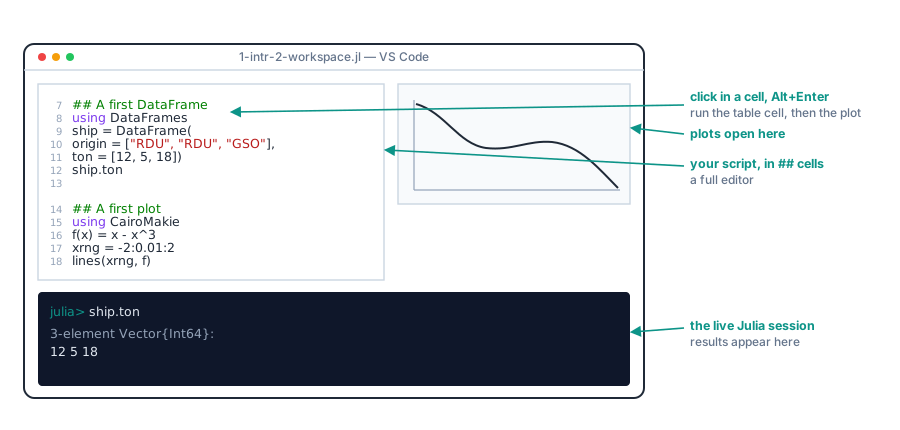
## cells; the live Julia session below it; and the plot pane on the right. Run a cell and its result appears inline and in the session, while a plot opens on the right.
Start a session. Open the .jl, then open the Command Palette from the menu bar (View ▸ Command Palette) and pick Julia: Start REPL. A julia> prompt opens in a panel below the editor. That panel is the live session for the whole file, and it stays warm throughout.
Run a cell at a time. A line beginning with ## marks the start of a cell, and the companion scripts put one example in each. To run one, click anywhere inside it and press Alt+Enter. The result shows up right next to the code and in the session below, and any plot opens in the plot pane on the right. That is the Jupyter feel, now inside a real editor.
Once the menus feel familiar, these are quicker. With the cursor in the editor:
The panel below the editor is a full Julia REPL, the same prompt a terminal would give. Toggle a plain terminal with Ctrl+** whenever one is needed. Typing **]** at thejulia>prompt switches to the package manager (the prompt turns topkg>`), and Backspace** returns to Julia. The next section uses package mode to get class-ready.
The tour matches the picture; the lecture’s full code lives in its companion script 1-intr-2.jl, opened and run the same way. Run its cells top to bottom and read each result as it appears; the very first, ## Get class-ready, installs the course’s packages, and Sec. 1.9 explains what it does.
Julia is a scripting language fast enough for engineering computation:
In interpretive languages like Python, MATLAB, or R, the fast operations are supplied by libraries written in C or C++, an opaque black box to whoever calls them. Julia reaches a speed comparable to C/C++ within Julia itself, so an implementation can be read all the way down rather than treated as a black box, which is exactly what verifying a result by reading its code requires.
The difference shows in practice: a simulation that runs in minutes under an interpreted language like Python can finish in milliseconds in Julia.
A further reason is visible in every lecture of this course: Julia identifiers can be the mathematical symbols themselves. A standard deviation can be named σ, an effective process time tₑ, a squared coefficient c², so the code reads like the formulas it implements. The symbols are typed as LaTeX-style abbreviations completed with Tab, in the REPL and in VS Code alike: type \sigma and press Tab to get σ; t\_e Tab for the subscript in tₑ; c\^2 Tab for the superscript in c². Operators come the same way: \div Tab gives ÷, integer division.
c² = σ² / tₑ ^ 2 = 4.03A cell shows only its last value: here 7 ÷ 2 prints 3, while the assignments above stay silent. @show overrides that for any line, printing the expression and its value; placed on a definition, @show c² = …, it inspects the result without repeating the name. A trailing ; silences even the last line, as Sec. 1.3 uses.
The course’s code uses such names throughout, so the same symbol carries from an equation in the prose to the variable that computes it.
Julia distinguishes integer and real scalars, and treats vectors and matrices as the 1- and 2-dimensional cases of an n-dimensional array:
n = 1 is an Int64 integer;x = 1.0 is a Float64 real;2×4 Matrix{Int64}:
1 2 3 4
5 6 7 8The last expression in a cell is displayed; ending a line with ; suppresses that. Case matters, so a and A are different variables. Several operators and functions build structured arrays:
6-element Vector{Int64}:
1
3
7
13
21
31A range like 1:5 is itself a compact one-element object used for iteration; the trailing ; inside [1:5;] is what expands it into a full vector. Writing collect(1:50_000_000_000) would instead try to materialize every element and exhaust memory. The last line is an array comprehension: [i^2 + i + 1 for i in 0:5] evaluates the expression once for each i in the range and collects the results into a vector.
Indices inside square brackets select elements. The colon : selects an entire row or column, and end is the last index:
a[3] = 12
a[[2, 4]] = [11, 13]
a[end] = 15A[1, 2] = 2
A[:, 1] = [1, 5]
A[1, :] = [1, 2, 3, 4]Ranges combine with end to slice off pieces, and reverse flips the order:
A scalar combines with each element of an array, but the operation must be broadcast with a leading dot. Multiplication is the exception, since * is already defined as scalar-times-array in linear algebra:
2 .+ a = [3, 4, 5, 6]
2a = [2, 4, 6, 8]
2a = [2, 4, 6, 8]Broadcasting expands a value to a compatible size, so 2 .+ a is the same as [2, 2, 2, 2] + a. The same dot turns any function elementwise, which is why so much Julia reads as a name, a dot, and an operator. Elements of one array are summed with sum and accumulated with cumsum; for a matrix, the dimension says whether to sum down columns or across rows:
sum(a) = 15
cumsum(a) = [1, 3, 6, 10, 15]sum(A, dims = 1) = [6 10 12]
sum(A, dims = 2) = [8; 20;;]When an array operation raises an error, the cause is almost always a missing broadcast dot; adding the . and running again resolves most such cases.
Comparing an array with a dot operator returns an array of true/false values, and the logical operators .& (and), .| (or), and .! (not) combine them. any and all reduce such an array to a single value:
a .> 0 = Bool[1, 0, 0, 1, 0]
(a .>= 0) .& (a .<= 4) = Bool[1, 1, 0, 0, 1]
any(a .> 0) = trueA logical array selects and changes elements just like an index array, and findall converts a logical array into the index array of the true positions:
a[a .> 0] = [5, 9]
findall(a .> 0) = [1, 4]Two more tools work on order rather than a condition: sort returns the values in order, sortperm returns the index array that puts them in order, and argmin (or argmax) gives the position of the smallest (or largest) element, the lookup behind finding a least-cost option.
sort(a) = [-1, 0, 0, 5, 9]
sortperm(a) = [3, 2, 5, 1, 4]
argmin(a) = 3Example 1: Selecting the heavy shipments
Five shipments have the weights below. Compute the line-haul charge at $50 per ton by broadcasting, then select the shipments heavier than 10 ton.
charge = 50 .* wt = [600, 250, 900, 350, 450]
heavy = wt[wt .> 10] = [12, 18]The charges are [600, 250, 900, 350, 450], and 2 shipments exceed 10 ton: [12, 18].
Arrays are mutable: elements can be added, removed, or changed. A tuple is similar but immutable, so once defined it cannot be changed; that guarantee lets Julia process it efficiently. A tuple is written with parentheses and indexed like an array:
t[2] = 1
typeof(t) = Tuple{Int64, Int64, Int64}Trying t[2] = 3 is an error, because a tuple is immutable. Tuples matter later because Logjam’s helpers read a shipment or carrier as a named bundle of fields, which is a tuple whose elements are named.
A tuple is like a toolbox drawer cut to fit each tool: fixed in size and layout, so its contents are found instantly. An array is more like a storage shelf. It can hold anything and can grow as needed, but an item takes longer to find unless its location on the shelf has been recorded; if not, the entire shelf must be searched. The tuple is built for efficiency, the array for flexibility.
The rest of this section is the one place the new course parts company with the 361 material. There, students wrote functions; here, the assistant writes them and the task is to read one well enough to check it and to trace a small case by hand. So the goal below is recognition, not authorship. The same small calculation, 3a + 1, is written first as a multi-line and then a one-line function, before an anonymous function, defined without a name, closes the section.
When the work takes several steps, or branches, a function is written on multiple lines between function and end, and hands back a value with return:
fun1(5) = 8.0The function can be traced by hand: with a = 5, b = 16, which is even, so c = 8.
When the body is a single expression, the same function fits on one line, with no function, return, or end:
Some functions take another function as an argument. filter is the classic one: given a predicate, a one-line function returning true or false, it keeps the elements for which the predicate holds. A named predicate works:
2-element Vector{Int64}:
12
18filter calls isheavy on each weight and keeps 12 and 18, the ones for which it returned true. But isheavy is a name spent on a test used once. This is where an anonymous function fits: written with -> (read “maps to”) in place of a name, w -> w > 10 is the same test with nothing to define, dropped straight into filter:
2-element Vector{Int64}:
12
18That is what a named function cannot do as cleanly, since it must be defined on its own line first. For a one-off predicate handed to another function, the anonymous form is the idiomatic choice.
Many results in the course reduce to solving \mathbf{A}\,\boldsymbol{x} =
\mathbf{b} for \boldsymbol{x}. Julia’s left-division operator \ does this directly, and the answer is verified by multiplying back.
Example 2: Solving and verifying a 3x3 system
Solve the system below for \boldsymbol{x} with the \ operator, then verify the solution by checking that \mathbf{A}\,\boldsymbol{x} returns \mathbf{b}.
\begin{aligned} 2x_1 - x_2 + 3x_3 &= 6 \\ x_1 \phantom{{}- x_2} + x_3 &= 3 \\ 4x_1 + x_2 + 8x_3 &= 17 \end{aligned}
3-element Vector{Float64}:
1.9999999999999996
0.9999999999999999
1.0000000000000002\boldsymbol{x} = [2,\,1,\,1], and \mathbf{A}\,\boldsymbol{x} returns [6,\,3,\,17] = \mathbf{b}, confirming the solve. Reproducing this check is exactly the kind of verification the course calls for.
Everything so far has used only base Julia, which is always available. The next two sections are the first to need a package: DataFrames for the table and CairoMakie for the plot. A package is installed once per machine, then loaded with using wherever it is first needed. Every package this course uses is installed together by the cell below, so a package that is new to a lecture is already on the machine, and Pkg.add is never the answer.
The companion script’s opening ## Get class-ready cell does the install. It finds the course project, activates it, and instantiates it, downloading every package at the version pinned for the course. It is safe to run repeatedly, so it need only run once per Julia session: activation lives in the running session, not in the file, so closing and reopening a script changes nothing, and only restarting the REPL or VS Code makes it necessary again. Unlike the rest of the lecture’s code, this cell is plumbing to run, not read: the walk-up loop and @__DIR__ are not course material, and there is nothing here to trace by hand.
# Code block 21: get class-ready, install the packages
import Pkg
let dir = @__DIR__
isproj = d -> isfile(joinpath(d, "Project.toml"))
env = d -> isproj(joinpath(d, "env")) ? joinpath(d, "env") :
joinpath(d, "materials", "env")
while !isproj(dir) && !isproj(env(dir)) &&
dir != dirname(dir)
dir = dirname(dir)
end
isproj(env(dir)) && (dir = env(dir))
isproj(dir) ||
error("no course project above $(@__DIR__)")
Pkg.activate(dir) # use the course project
Pkg.instantiate()
endProject.toml turns up, either in that folder, in an env/ beside it, or in a materials/env/ beside it; that folder is the course project. Three places, because the course keeps it in three: at the top of the repository these pages are built from, under env/ in the materials repository a student clones, and off to the side in materials/env/ as seen from a script copied into work/.
activate on a folder holding no Project.toml quietly creates an empty environment, instantiate reports success, and the first using fails much later for a reason that no longer looks like this cell.
instantiate reads the Manifest.toml and installs every listed package at its exact pinned version, skipping any already in place.
Project.toml and Manifest.toml are
A Julia project is just a folder with two files. Project.toml lists the packages the project depends on, by name. Manifest.toml records the exact version of every one of those packages, and of everything they in turn depend on, so instantiate can rebuild an identical environment on any machine. The course ships both, which is why everyone runs the same versions and results match the lecture’s.
A package’s functions become available once it is loaded with using. Rather than load everything at the top of the file, this lecture brings each package in right where it is first needed, so it is clear which section depends on what: using DataFrames opens the next section, and using CairoMakie the one after.
A DataFrame holds tabular data in named columns of equal length, the table form the rest of the course composes for transport, location, and inventory calculations. A table is built by naming its columns and a column is read back with dot notation:
Example 3: A small shipment table
Assemble a three-row table of shipments, each with an origin, a destination, and a weight, then read back the weight column.
| Row | origin | dest | ton |
|---|---|---|---|
| String | String | Int64 | |
| 1 | RDU | ATL | 12 |
| 2 | RDU | MIA | 5 |
| 3 | GSO | ATL | 18 |
ship.ton is the 3-element vector [12, 5, 18], the weights pulled straight out of the table by name.
A language for engineering has to draw, and Julia draws as readily as it computes. A single command turns a function into a figure, and that same command takes keywords for a title and axis labels, so the plot is presentable without any extra setup:
lines draws f over the range xrng; the axis = (...) keyword sets the title and axis labels inside the same call, so the separate Figure and Axis objects that fuller plots use are not needed yet.

lines call.
lines here comes from Makie, a full plotting system for Julia. Makie has several backends: CairoMakie renders static, publication-quality images (PNG, SVG, PDF) and is what this course uses for figures on the page; GLMakie opens fast interactive windows; WGLMakie targets the browser. A popular alternative family is Plots.jl, which wraps several plotting libraries behind one simpler syntax. For this course, CairoMakie is all that is needed.
That single lines call is the whole of it. Drawing several series together, adding a legend, and arranging multi-panel layouts come in later lectures; here one curve is enough to show that plotting is one command away.
A language model does one small thing: predict the next token, over and over. Everything else, including how it is steered, is built on that single move.
AI assistant tools like Claude Code are based on large language models (LLMs). This section is not a comprehensive introduction to LLMs. Its job is narrower, and it has two parts: to provide the reader with a mental model accurate enough that LLM-based tools can be used effectively, and to make clear why the output of those tools has to be checked at all. The analogy is driving. To drive effectively, an engine schematic is not needed, the driver needs to know only the physics of steering. In an LLM-based tool, the engine is next-token prediction, and the steering wheel is the context window. The one idea runs through everything that follows: steering acts on what the model can see, not on what it knows.
Driving is not the whole of it. This course asks not only that the tool be steered but that its answer be judged, and that is a question about what the engine can and cannot do. Secs. 2.2 to 2.6 open the hood: how a window of tokens becomes a next guess. They are here because the reason a language model can be fluent and wrong at the same time is visible in the mechanism and nowhere else. Knowing it turns “check the output” from a rule to be obeyed into a conclusion that can be reached.
Strip everything away and a language model does one small thing: it reads the tokens in front of it, predicts the most likely next one, adds it to the end, and does the whole thing again. A token is a chunk of text, roughly three quarters of a word, and the tokens the model can see at this moment are its context window, the whole of its working memory for the task.
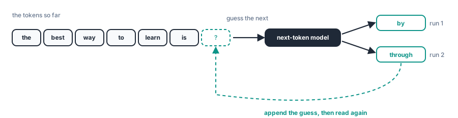
The prediction is a guess, not a lookup. The model samples from a range of plausible next tokens rather than always taking the single likeliest, so the same prompt can finish “the best way to learn is by doing” on one run and “through failure” on the next, as Fig. 3 shows.
The striking part is how little machinery it took to learn this. The model trained itself on a self-checking game played at enormous scale: take ordinary text, hide the next token, guess it, and compare against the word that was actually there. Text is its own answer key, so no human had to grade it. The jump in capability over the past few years came not from a clever new idea but from running this plain game over far more data and computation, the point Richard Sutton called the bitter lesson.2
Two questions remain, and they organize the rest of the reading: how does the model turn a window of tokens into a good next guess, and how is that guess steered? We take them in turn.
The first thing that happens to the text is that it stops being text. Each token is looked up in a large table, and what comes back is not a piece of a word but a long list of numbers, often 768 of them, called the token’s embedding, the fixed vector the model stores for that token.
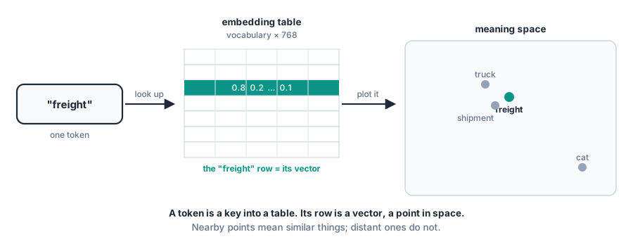
Read those numbers as coordinates and every token becomes a point in a high-dimensional space, arranged during training so that tokens with related meanings land near one another. Nearness is meaning. Fig. 4 shows the idea in two dimensions, where “truck”, “freight”, and “shipment” cluster while “cat” sits far off. It is also why everything about these tools is counted in tokens, context limits, speed, and cost alike: the token is the unit the whole machine moves around.
A small example makes the geometry tangible. We place a few words by hand and measure how related two of them are straight from their coordinates.
Example 4: A token as a point in space
Represent a few words as points in a small space, then measure how related two of them are using only their coordinates.
Each word is one column of a matrix, a point in two dimensions where a real model would use hundreds. A word’s vector is the column its key selects. Relatedness is the cosine of the angle between two vectors: near 1 when they point the same way, near 0 when unrelated, and negative when opposed.
# Code block 25: tokens as points in a space
vocab = ["truck", "freight", "shipment", "cat"]
# E: one column per token, each a point in 2-D meaning space
E = [0.9 0.8 0.85 -0.7
0.1 0.2 0.05 0.9]
emb(w) = E[:, findfirst(==(w), vocab)] # token -> vector
cosine(a, b) = (a'b) / (sqrt(a'a) * sqrt(b'b))
@show cosine(emb("truck"), emb("freight")) # related
@show cosine(emb("truck"), emb("cat")); # unrelatedcosine(emb("truck"), emb("freight")) = 0.9909924304103231
cosine(emb("truck"), emb("cat")) = -0.5230162198525903-0.5230162198525903The ' in a'b is the adjoint (transpose): it lays the column a on its side, so a'b multiplies and sums the two vectors elementwise, the dot product \sum_i a_i b_i. Section 2.3 uses the same '.
The cosine of truck and freight is \approx 0.99 (closely related); of truck and cat, \approx -0.52 (unrelated). The coordinates alone carry the meaning.
Every later step is geometry on points like these: combine them, compare them, and read off the nearest. How much combining a prediction needs is the thread of the next three sections, which take it in three steps: the next token can depend on a single token, on a fixed combination of tokens, or on a combination the model must pick out by content, and these three are answered in turn by a single layer, a hidden layer, and attention.
Sections 2.1 and 2.2 gave the model its input: the tokens so far, each turned into a point in space. The prediction is a choice among the whole vocabulary, which token comes next. Choosing one option from a fixed set is classification, and it is the task that runs all the way to attention, so we build it from the ground up.
What follows is a machine assembled from elements called neurons, each with a set of adjustable numbers. Training it means tuning those numbers until its answers fit a collection of examples, the same idea as fitting a straight line to data by choosing the slope and intercept that make the errors smallest. The adjustable numbers here are called weights and biases: the weights play the role of the line’s slopes and the biases its intercepts, and the machine is built from one repeated building block called the neuron.
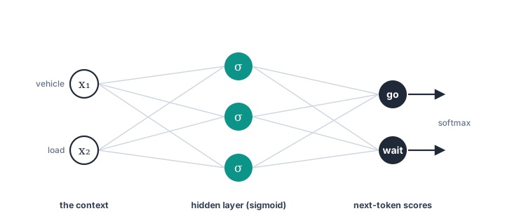
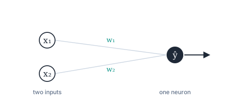
A neuron multiplies each input by a weight, sums them with a bias, and passes on the total, a weighted sum w_1 x_1 + w_2 x_2 + b (Fig. 5). The bias is the intercept; without it the sum is zero whenever the inputs are, so the bias sets a baseline while the weights set the response. One neuron gives one score. To score every candidate token we use one neuron per token, all reading the same input, and that bank of neurons is a layer, the simplest neural network there is. It turns a token’s embedding into a list of scores called logits.
A logit can be any size or sign, so it is not yet a probability. The softmax makes it one: raise e to each score, so larger scores pull ahead, then divide by the total so the results are positive and sum to 1.
\text{softmax}(z)_k = \frac{e^{z_k}}{\sum_j e^{z_j}}.
Now the layer outputs a probability for every possible next token, the distribution it samples from, and it is the same softmax Section 2.5 uses to place attention. In base Julia, written to act on each column so it can score many tokens at once:
round.(softmax([2.0, 1.0, 0.0]); digits = 3) = [0.665, 0.245, 0.09]Training tunes the weights by gradient descent, minimizing a cross-entropy loss whose gradient reduces to the P .- Y in the loop below.
Training tunes the weights by gradient descent, a familiar idea: follow the slope of a loss downhill. What should the loss be? A good model makes the real data likely, putting high probability p_t on the token that actually came next. The chance it assigns to the whole corpus is the product of those p_t, and a logarithm turns a product into a sum, so making the data likely is the same as minimizing L = -\log p_t added over the examples. That loss is cross-entropy.
Its form earns itself twice over. The shape of -\log is exactly right: zero when the model was sure and correct, with p_t = 1, and rising without bound as p_t \to 0, so a confident mistake costs the most while an honest hedge costs little. And its slope is as clean as a straight line’s: the correction to the scores is the predicted distribution minus the target, p - y, where the target y marks the true token with a 1 and the rest with 0. That difference is the P .- Y in the loop.
The simple gradient p - y is a standard result of pairing cross-entropy with softmax, quoted here rather than derived.
Example 5: Predicting the next token by gradient descent
Place a few tokens as points in a two-dimensional space, give a tiny corpus in which the current token determines the next, and train a single layer by gradient descent until it predicts the next token correctly.
The training data is a corpus. In a real one the examples are carved from running text: at each position the tokens before are the context and the next token is the target, so a passage yields an example at every step, the self-checking game of Section 2.1 across trillions of tokens scraped from the web. Ours is seven examples by hand, each a two-token sequence like van go or depot wait, the context first and the target second. Table 1 lists them in full.
| context token | next token |
|---|---|
van |
go |
rig |
go |
parcel |
go |
pallet |
go |
depot |
wait |
yard |
wait |
dock |
wait |
Now we let gradient descent learn the embeddings too. The tokens start at random points, and the same loop that tunes the readout also slides each token, so the cargo words drift together on one side and the place words on the other while the boundary settles between them. This is the training of Section 2.2 in miniature, and it shows the embeddings are not a separate, earlier stage: the table is just more parameters, moved by the same gradient descent against the same next-token loss as the readout, all in one motion. The tokens cluster by meaning not because the model is told what words mean, but because that arrangement is what lowers the loss. In the code the embeddings are the matrix E, the pairs become ctx and nxt, and the loop updates E along with W and b.
Each of the 4000 passes computes the predictions, measures the error P .- Y, and nudges the readout weights, the biases, and the embeddings one learning-rate (lr) step downhill.
# Code block 27: training the next-token model
using Random
vocab = ["van", "rig", "parcel", "pallet",
"depot", "yard", "dock", "go", "wait"]
id(w) = findfirst(==(w), vocab) # token -> column
# corpus: each context token -> the next token
ctx = ["van", "rig", "parcel", "pallet", "depot", "yard", "dock"]
nxt = ["go", "go", "go", "go", "wait", "wait", "wait"]
V = length(vocab); N = length(ctx)
cols = id.(ctx) # context columns of E
Y = zeros(V, N) # one-hot targets
for j in 1:N
Y[id(nxt[j]), j] = 1
end
# E: a 2-D embedding per token, learned from scratch
Random.seed!(1) # same starting points every build
E = 0.4 .* randn(2, V)
W = zeros(V, 2); b = zeros(V, 1); lr = 0.5
for epoch in 1:4000
X = E[:, cols] # current embeddings
P = softmax(W * X .+ b) # next-token probs
dZ = P .- Y # cross-entropy gradient
dX = W' * dZ # error back to embeddings
W .-= lr .* (dZ * X') # readout weights
b .-= lr .* sum(dZ, dims = 2) # readout biases
E[:, cols] .-= lr .* dX # move the embeddings too
end
pred(c) = vocab[argmax(W * E[:, id(c)] .+ vec(b))]
@show pred.(ctx); # all seven correctpred.(ctx) = ["go", "go", "go", "go", "wait", "wait", "wait"]In Julia a dot makes an operation elementwise, so W * X .+ b takes the matrix product W * X and adds the bias to every column; a plain * is matrix multiplication and ' transposes, so dZ * X' sums the gradient over all N examples at once.
After training, the tokens have pulled apart into a cargo cluster and a place cluster, the layer sends every cargo word to go and every place word to wait, and the cross-entropy loss falls to about 0.
It is worth seeing where the straight line in Fig. 6 comes from, since the model only ever computed scores. The model predicts go for any input whose go score beats its wait score, and wait otherwise; the border between the two verdicts, where the scores tie, is a straight line because each score is a flat weighted sum of the coordinates. Training works both ends at once: it slides the token points until the two classes pull apart, and it swings that boundary until the go words sit on one side and the wait words on the other.
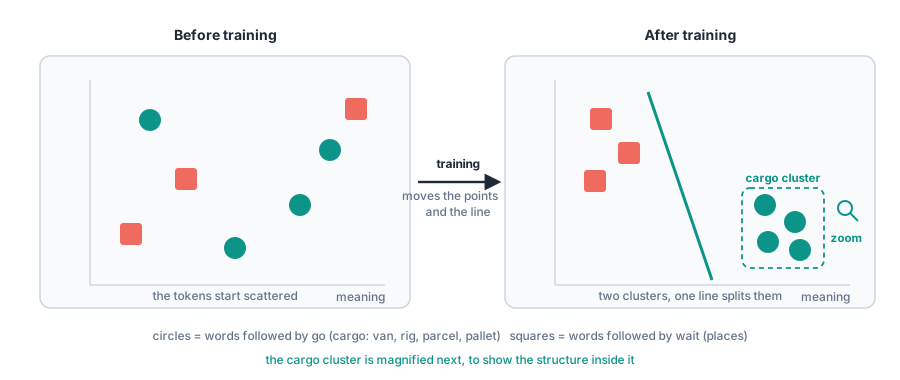
Notice what made one layer enough here. With the embeddings free to move, the model can place each token wherever it likes, and when a single token determines the next, that freedom is the entire solution: arrange the points, draw one line, and every case is covered, with nothing left for a deeper network to do. That is the condition Section 2.4 breaks.
Attention is the operation that lets each token gather meaning from the others before the readout of Section 2.3 runs; it is the third and last step.
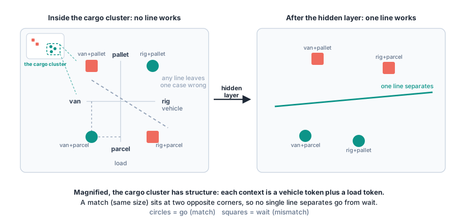
The hidden layer combined two tokens, but only because we promised which was which: token one the vehicle, token two the load. Language never makes that promise. The token a word depends on may sit anywhere, and which token it is changes with the content, not the position. So the combination cannot be wired in ahead of time; the model has to work out, for each token, which others matter to it. Attention is that operation, and it is the third step: where the hidden layer computes how a fixed pair of tokens interact, attention also computes which tokens interact.
Take “the truck left because it was full.” On its own, “it” means almost nothing. Attention lets the vector at “it” look back over the window, score how well each earlier token answers what it is looking for, and pull in meaning from the ones that match, here mostly “truck”, so that afterward the vector at “it” has come to stand for the truck. The same word among different neighbors comes out a different vector.
Example 7: Attention resolves a reference by content
Give a token a query, score it against the earlier tokens by content, and blend them into a new vector for that token, using nothing but base Julia.
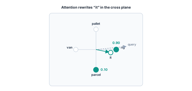
The model is about to predict after it, in a window where it refers to the rig. The token forms a query, a learned view of itself that says what it is looking for; here that query points toward the rig. Each earlier token is scored by how well it matches the query, a plain dot product, and the softmax of Section 2.3 turns those scores into weights.
# Code block 29: attention weights for one query
q = [2.0, 0.2] # the query "it" forms
rig = [1.0, 0.0] # the same cross points
parcel = [0.0, -1.0] # from Section 2.4
s = [rig' * q, parcel' * q] # match each by content
w = softmax(s) # weights, positive, sum to 1
it = w[1] .* rig .+ w[2] .* parcel # blend into a new vector
@show round.(w, digits = 2); # most weight on the riground.(w, digits = 2) = [0.9, 0.1]About 0.90 of the weight lands on the rig, so the rewritten it comes out close to the rig’s own vector, (0.9, -0.1): it now carries the rig’s meaning. The match was made by content, the query against each token, not by any fixed slot; move the rig elsewhere in the sentence and the same query would still find it.
That is the whole of attention. It rewrote one token into a better vector by gathering from the tokens it judged relevant, and from there the readout of Section 2.3 reads the next token off that vector exactly as before. Attention does not replace the machine of the earlier sections; it hands that machine a token whose meaning already reflects its context. The weights are a softmax, so each token has a fixed budget of attention, positive and summing to 1, and leaning harder on the rig means leaning less on the rest, a limit Section 2.7 returns to.
Those are the three steps the next-token prediction takes. The next token can depend on one token, read off by a single layer; on a fixed combination of tokens, computed by a hidden layer; or on a combination chosen by content, computed by attention. A real model is these three, stacked and scaled. Interleave attention with per-token layers like Section 2.3’s, many times over, and that stack is a transformer; scale it up and train it on the next-token game of Section 2.1, and the result is a language model.
The shape rules from Sections 2.4 and 2.5 explain much of the size. Each layer now carries a token’s full embedding from Section 2.2, so it must be at least as wide as that embedding, hundreds or thousands of neurons rather than three; and the output layer is no longer one neuron but one for every token in the vocabulary, tens of thousands of them. Stack those wide layers many deep and the weights run into the billions.
When the model runs, that output layer emits one logit per word in the vocabulary, the raw scores of Section 2.3, and the softmax introduced there turns the whole list into the probability distribution the model samples its next word from, the guess of Section 2.1 at full scale.
The weights are set in two stages. Pre-training minimizes next-token cross-entropy across much of the public web, the self-checking game of Section 2.1 made quantitative, and builds raw capability. Every weight moves under that single objective at once, the embedding table from Section 2.2 included. Fine-tuning then shapes how the model uses that capability, and it has two parts of its own. Supervised tuning on example dialogues teaches it to follow instructions. Then reinforcement learning tunes it by reward rather than by example: the model produces an answer, the answer is scored, and the weights shift to make higher-scoring answers more likely. At first the score came from human preferences, people choosing the better of two replies, known as reinforcement learning from human feedback. Increasingly it comes from automatic checks of whether an answer is actually correct, a unit test that passes or a math result that matches, which is much of why recent models improved so sharply at code and reasoning. It is the same verifier idea that closes the agent loop in Section 2.10, moved to training time. One side effect matters later: when the reward favors giving an answer over admitting uncertainty, the model learns to do exactly that. After fine-tuning the weights are frozen, and they do not change during use.
So the engine is sealed. The one thing that changes at run time is the context window, the tokens the model can see right now. Everything provided, instruction, example, file, tool result, lives there, and nothing else does.
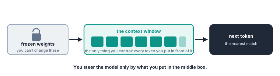
Fig. 10 is the whole reading in one picture. From here on we stay in that middle box. We have already seen why its contents matter so much: attention reads every token in the light of the others. What remains is that the window can be filled well or badly, which is where the controls begin.
The fixed budget has a cost. Because each token’s attention sums to 1 no matter how many tokens share the window, a longer window slices the same budget thinner, so every token gets less notice. And the budget is not spread evenly.
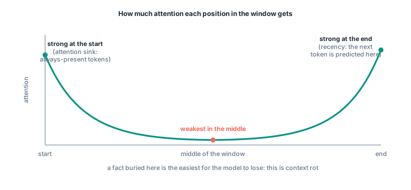
Fig. 11 shows the shape, and it is not arbitrary.3 The end wins because predicting the next token is the whole job, so the most recent tokens weigh most, and a token’s influence fades with distance in any case. The start wins for a subtler reason that falls straight out of the budget: since the weights must sum to 1, the model always has a full unit of attention to spend even when nothing is especially relevant, so it learns to park the surplus on the first few tokens, which sit at a fixed spot and are seen by every later token. Those become an attention sink.4 The middle gets what is left, which is why a detail buried there is the easiest to lose. The shorthand for the whole effect is context rot.
Two working habits follow. Keep the window relevant and well ordered; more text is not more understanding. And put any instruction that must hold all session where attention is strong, then restate it as the window grows, since one buried mid-window quietly loses force.
Relevant is not the same as short, and the difference determines how a session is run. Every prediction is weighed against everything else in the window. A session that has stayed on one problem offers a small, consistent set of things to weigh, and it does well. A session that has wandered across three problems, two dead ends, and a file opened by mistake offers a much larger and less consistent set, and every prediction now has to account for all of it. The instruction that matters is still there. It is simply competing with far more than it was an hour ago.
So length by itself determines nothing. An hour spent on a single location model is an hour of useful context: the model holds the column names, the two approaches already ruled out, and the error hit twice. Starting fresh discards all of it, spends ten minutes rebuilding it, and may repeat a mistake already eliminated. An hour that drifted from a plot to a routing calculation to a file opened by mistake is the opposite, since almost none of it bears on the current question and all of it still competes. The test is not how long the session has run but whether what is in the window is about what is being asked. When that stops being true, start a new one.
The same mechanism is also a gift. Drop two or three worked examples into the window and the model copies the pattern, with no change to its weights, simply because attention conditions its output on what it can see. This is in-context learning, the cheapest steering available: show, do not only tell.
In-context learning shows what the window can do; context rot shows what it cannot guarantee. An instruction can always slip as the window fills, so when a rule truly must hold, the move is to take it out of the window and put it in code that runs around the model and checks every action, however cluttered the context. That code is a hook. It is the gate in Fig. 13 further on: every action the model proposes passes through the hook, and only a passing check lets it through.
Those actions have a name. Everything the model does beyond producing text, reading a file, writing one, running a command, searching the web, is a tool call: the model does not reach out and act, it requests an action from a fixed list its environment offers, and the environment performs it and reports back what happened. A tool is one entry on that list, and it has a name, such as Edit, Write, or Bash. Two things follow, and the second is what makes this section possible. The list is fixed, so what the model can do at all is determined by whoever assembled the environment, not by the model. And because every action arrives as a request rather than as a deed already done, there is a moment between the asking and the doing. That moment is where a hook sits.
In a tool like Claude Code a hook is set in a settings file by pairing an event with a command. Events are points in the model’s loop, before it runs a tool, after it edits a file, when a session starts; the command is an ordinary shell command, and an exit code of 2 blocks the action it guarded. Attach to “after a file edit” a run of the test suite, julia --project -e "using Pkg; Pkg.test()", and a failing test rejects the edit; attach a formatter and every touched file comes back tidy; attach to “before a tool runs” a check that refuses edits to a protected data file. The model cannot argue its way past any of these, because they are not instructions it must remember but code that runs no matter what it does. When a guarantee matters, write it as a hook, not as a sentence in the prompt.
A worked example. Suppose one file is not the assistant’s to touch, an answers.txt holding work that has to be the reader’s own. As an instruction, that can slip as the window fills; as a hook, it cannot.
Hooks are set in a settings file. Claude Code reads .claude/settings.json from the folder the session was started in, so what it says applies to that project alone.5 For this course that folder is ISE754, the one holding materials/ and work/, and the file is already there: the setup put it in place, carrying the permission rules that let routine commands run without asking each time. A hook is another entry in the same file. Because the file sits in the project folder, it travels with the folder, so a rule written once is in force for anyone who has a copy.
.claude/settings.json
PreToolUse is the event that fires before a tool runs, and matcher picks which tools it guards, here the two that modify files. The command can be any program at all. This one is five lines of shell, and it is the entire rule:
.claude/hooks/protect-answers.sh
The hook is handed a description of the action the model proposes to take. grep is the standard command for searching text for a pattern, and the -q flag asks it to report only whether the pattern was there rather than printing what it found, which is all a yes-or-no decision needs. If answers.txt appears anywhere in it, the hook prints a reason and exits 2; otherwise it exits 0 and the action goes ahead. Searching the whole description is deliberately crude: it would also stop a file that merely mentions that name, and it does not care which folder the file is in. A real rule would read the path out of the description instead, but the point here is the mechanism rather than the matching. Exit 2 is the code that blocks, and it is the one to get right: any other nonzero code counts as the hook itself having broken, so the action is allowed through, which is the reverse of what a rule like this intends.
A block is not a failure the reader has to deal with. The reason goes to the model rather than to the reader, and the model reads it as an attempt that did not work and tries another way, most often the right one: a different file, or a question. So a hook behaves less like a wall than like a harness. It keeps the assistant inside the lines, and it does so without asking anything of the reader.
Three things follow from the shape of it. The rule holds whether or not the model remembers it, since nothing was asked of the model at all. It holds identically on the hundredth turn and the first, so context rot cannot erode it. And it is legible: the guarantee can be checked by reading five lines, which is not true of an instruction competing for attention somewhere in a long window.
A hook can stop a bad action, but it cannot make the model know something it does not. Because the model must emit some next token at every step, it can never answer that nothing fits. When a good continuation sits close by, the nearest match is the right one. When nothing good is near, the model returns its closest token anyway, and it sounds exactly as sure as when it is right.
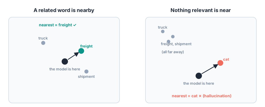
That is a hallucination, and Fig. 12 carries the lesson: confidence says nothing about correctness. Ask for a logistics term with “freight” close at hand and the answer is “freight”; ask where nothing relevant is near and the answer may be “cat”, delivered with the same certainty. A made-up Julia function with a plausible name reads just like a real one. Models are, if anything, trained to prefer a confident guess to an honest admission of not knowing, because on most tests a guess outscores an abstention.6 Treat fluency as fluency, never as evidence.
If a hallucination is the absence of a good answer nearby, the cure is to put a good answer in the window. That is what tools are for. Web search drops current facts in front of the model; a code sandbox runs what it wrote and returns the real result; access to the working files hands it the actual code and data. Each one trades a guess from frozen weights for ground truth set in view.
This gives the cleanest definition of an agent: a language model whose context window is managed by its environment instead of by a person typing. A chatbot waits for a person to add tokens by hand; an agent acts, the environment feeds the result back into the window, and the cycle repeats. The range runs from the prompted chatbot, to a coding agent looping toward a set goal, to an autonomous agent following defined rules.
The loop turns powerful the moment it can tell whether it is done. Give the model a checkable goal, a unit test, and it can run unattended: propose code, run it, read the failure, fix it, and go again until the check passes.
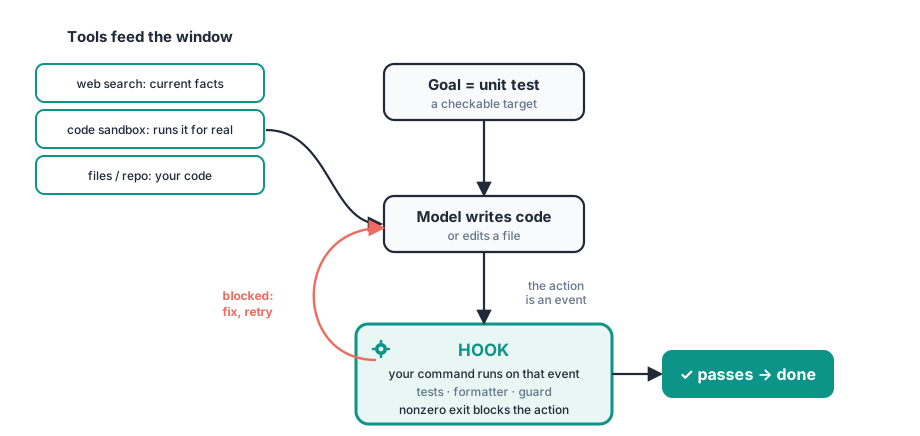
Fig. 13 is that cycle, with a hook as the gate that runs the check on every pass. It is the Ralph Wiggum loop, after the Simpsons boy who keeps trying and grins “I’m learnding”: it converges by sheer iteration, without needing to understand why. It also explains why coding ran ahead of almost everything else these tools touch. Software already carried its verifier, the test suite, long before AI arrived, and the public web is full of code paired with tests. Where a cheap check exists, as in code and mathematics, the loop closes and progress is fast; where “correct” cannot be machine-checked, the loop has nothing to close on, and the scarce human skill becomes verification itself.
Everything so far steers a fixed model through its window. One last lever changes the weights themselves. Open-weight models publish their weight files, so they can be fine-tuned them on local data and run them on local hardware, even a single desktop GPU; closed models can only be prompted, or fine-tuned through a vendor without ever holding the weights. For an engineering group the difference is real: open weights allow specializing a model to a domain and notation, keep proprietary data on local machines, and adjust its disposition rather than only its window. Mechanically it is no new machine: fine-tuning is the same gradient descent as Section 2.3 with the weights unfrozen, nudged on local examples by cross-entropy or by the reward of Section 2.6. Steering the window is the daily work; changing the weights is the lever held in reserve for when the window is not enough.
Sec. 2.7 showed the window to be finite within a session. It is worth being clear that it does not survive one either. A language model holds no state between sessions: the weights are frozen, and the window is emptied. What looks like memory in a tool like Claude Code is a file being read back into the window at the start of the next session, so a tool that appears to remember a project is one that re-reads it.
Two consequences follow, one practical and one sharper. The practical one is that anything which must survive has to be written down in the project rather than left in the conversation. Instructions meant to apply to every session belong in a file the tool reads on startup; a decision reached after an hour of argument belongs in a note, or it will be argued again next week.
The sharper one is that a session summary is not a record of the past session, it is the context of the next one. Its quality is the next session’s competence. A summary naming what was determined, what was tried and rejected, and what is still open puts the following session where this one ended. One that says “worked on the location model” starts it from nothing, and the hour spent ruling out two approaches is spent again.
So the move at the end of a working session is to ask for a summary, and then to read it. Asking is cheap. Reading is the part that matters, because a summary is a claim about what happened, written by the same machine whose claims arrive with unearned confidence (Sec. 2.9). A summary that has quietly dropped the constraint which took an hour to establish reads exactly as smoothly as one that kept it, and the cost of the omission is not paid until next week.
The assistant writes the note; the reader checks it. That division is the same one the whole course runs on, and it applies here for the same reason: the assistant has the session in its window and can summarize it in seconds, while nobody else can tell whether the summary is faithful. So the habit at the end of a working session is one instruction. Take the occasion most likely to come first: the setup of Sec. 1 is part done, a package is still precompiling, and the session has to stop for the evening. One instruction at that point,
Write a handoff note to
handoff.md: where this stands, what was determined and why, what was tried and rejected, what is still open, and the next step.
which returns something along these lines:
handoff.md
# ISE 754 setup handoff, 18 Aug
## Where this stands
Julia 1.12.6 and VS Code are installed and working, and the course
materials are cloned to Documents/ISE754/materials.
## Determined
Installed Julia through juliaup rather than the standalone installer,
so the course version can be pinned without disturbing the Julia 1.11
already on this machine.
## Tried and rejected
Running the check from the home folder. It has to run from inside the
materials folder, and the error it gives there does not say so.
## Open
The check does not report READY yet. One package is still precompiling.
## Next step
Re-run env/bootstrap_check.jl and read the first failing line.Then read it. Two of those five headings are the ones worth reading closely, because they are the ones that cost real time to rebuild: Determined, which is a claim about a judgment, and Tried and rejected, which is the time that need not be spent again. A note whose Determined section has quietly lost the reason attached to the decision looks complete and is not.
A file answers what the state is now. It does not answer what changed, and the change is often the question. That is what a version-control system is for, and this course keeps its material under one, git. Because git stores a project’s history rather than only its present, a session can be handed the revision instead of the current text:
Show me how the Determined section of
handoff.mdchanged over the last three commits, and tell me whether anything was dropped.
The assistant answers that with git log and git diff rather than with recollection, and the difference matters: a decision that was reversed leaves a trace in the history and none at all in the file. Reading evidence is not the same as being told a story, and it is why a handoff note is worth committing rather than merely saving.
Committing is also what makes one note enough. handoff.md keeps its name and is overwritten at the end of each session, because overwriting a committed file loses nothing: every earlier version is in the history, reachable by date or by commit. The same habit without version control needs handoff-18-aug.md sitting beside a dozen siblings, and a folder of near-identical notes is worse than a single current one, because the first task becomes working out which is live.
“Trust, but verify.” (“Doveryai, no proveryai.”)
— Russian proverb, quoted in Russian by Ronald Reagan at the signing of the 1987 INF Treaty. Gorbachev: “You repeat that at every meeting.” Reagan: “I like it.”7
The three parts of this lecture were introduced as meeting on one idea: the assistant writes the Julia and the reader verifies it. This closing part is about verification: why it is now a skill in its own right, the nine named checks the course uses to practice it, and the form an analysis must arrive in so the checks have something to grip. Table 2 collects the nine on one card, each with a short example to keep in mind; Lecture 1.3 puts them to work on real systems.
The course’s modeling workflow divides the work three ways:
In Balaji Srinivasan’s phrase, “AI is not end-to-end but middle-to-middle”: the human owns both ends, the intent in front and the verification behind, while the assistant owns the middle. In course terms, the assistant writes the Julia and the human answers for the result. That division of labor is why validation, once a skill nobody had to teach, is now the one this course grades. Three things changed:
None of this makes validation new; checking has always been part of good engineering practice, and a fair question is why a logistics course suddenly makes so much of it. The honest answer is that there was never room before: when every model and every line of code had to be built by hand, getting a working system at all consumed the course, and checking stayed implicit in the labor of construction. Think of it as building an airplane. Before AI assistance, the achievement was a plane that could get off the ground at all, and the course was spent building it; with an LLM-based assistant, the plane always gets off the ground, so the time goes where it always should have gone, to testing whether it is airworthy. Validation is not new under the sun; what is new is a course with room to teach it.
There is a catch, and it is why the verifying end cannot be waved away. “… even if LLMs end up replacing a lot of knowledge work, it’s good to know things and in particular good to have exceptionally deep knowledge in some domain,” Byrne Hobart observes. “How good you are at the thing you’re best at determines how powerful an LLM you can reasonably evaluate. If Grok is twice as good at physics as I am, but OpenAI is three times as good, I’ll have no way of knowing.”8 Verification reaches only as far as the knowledge behind it; the logistics this course teaches is what gives the checks below their teeth.
The good news: checking is fundamentally easier than creating. Verifying a completed Sudoku takes a minute of scanning; filling the grid can take an evening. Computer science makes the asymmetry precise, in the verified-quickly versus solved-quickly gap on which the P versus NP question turns,9 and mathematics has known it for centuries. “Every person is capable of judging a proof,” Leibniz wrote in 1677; “nevertheless, not everyone is capable of discovering proofs independently.”10 The side of the work left to the human is the tractable side.
One rule governs every check that follows: independent and cheap. Re-reading the assistant’s explanation is not a check, and neither is asking the model whether it is sure; both draw on the same source as the error they are meant to catch.
The lecture’s epigraph names the stakes; meeting them means holding both ends of the workflow: understanding reasonable objectives and practical constraints in front, and verifying the results behind. The analysis and the computing do not go away.
The checks come in three families of three, ordered by the effort they cost. Screens run in seconds, on every result. When a result is used, feeding a next step, one expectation is added. When a result is signed, submitted or relied on by someone else, one confirmation is added. Every validation ends in a verdict: accept, reject, or escalate to a better check. Never a feeling.
| Family | Check | Asks | Example |
|---|---|---|---|
| Screens | Units | Do the units work out? | Pizza delivery |
| Bounds | Does it break a hard limit? | Bathtub | |
| Assumptions | Are the preconditions met here? | Spherical cow | |
| Expectations | Prior | Does it land inside the estimate committed before the run? | Guesstimate |
| Nudge | Does the answer move the right way? | Hotel shower | |
| Landmark | Does it hit a case already known? | Home to home | |
| Confirmations | Triangulate | Does an independent route agree? | Two lighthouses |
| Balance | Do the parts add up to the whole? | Restaurant bill | |
| Source | Does the document say what is claimed? | Scrabble |
Screens run on every result, always, and cost seconds; a failed screen ends the matter with a reject before any deeper check is spent.
Units. Do the units work out? Miles divided by miles-per-hour must come out in hours: the 10-minute pizza delivery that Lecture 1.3 works out is 4 mi at 24 mi/hr, and had the division produced anything but time, the formula, not the arithmetic, would be wrong. Multiplying the units through a formula and confirming the answer carries the unit the question asked for is the fastest check there is, and the stakes can be real: in 1983 an Air Canada 767 ran out of fuel at altitude because its fuel load had been computed in pounds where kilograms were required, and the crew glided it onto a drag strip at Gimli, Manitoba.11
Bounds. Does the answer break a hard limit? A bathtub whose faucet runs faster than its drain will overflow, and no cleverness about how the water is poured changes that. A probability above one, a trailer loaded past its rated capacity, a negative waiting time: an answer on the wrong side of a hard limit is wrong regardless of the reasoning that produced it. (Lecture 1.3 turns this bathtub into the utilization condition of a queue.)
Assumptions. Are the formula’s preconditions met by this instance? In the old physics joke, a theorist solves a dairy farm’s troubles beginning “assume a spherical cow in a vacuum”: the model is exact, and useless, because its fine print fits no actual cow. Every formula carries fine print the same way, and the check is to read it against the situation at hand before trusting the number. The models of Lecture 1.1 state their assumptions for exactly this reason.
Expectations compare the answer against a reference the checker supplies, the one part of the work no assistant can do. One expectation is added whenever a result is used, feeding a further step: the prior if one was committed, otherwise a nudge or a landmark, which still work after the fact.
Prior. Does the answer land inside an estimate committed before the answer was seen? This is the guesstimation of Lecture 1.1, repointed: bracket the quantity between a low and a high, take the geometric mean, and write it down before the assistant runs. The skill that produced answers when nothing better was available now guards the answers something better produces. The timing is the whole check: the county-fair jelly-bean guess is sealed before the answer card is turned over, because a guess written afterward is no guess at all; an estimate stated after seeing the answer is a posterior and checks nothing. Fermi’s paper scraps were exactly this, an estimate of the blast that existed before the instrument readings arrived.12
Nudge. Push an input; does the answer move the right way? In an unfamiliar hotel shower, turning the handle toward red while the water runs colder proves the plumbing is crossed, without knowing what the right temperature is. The check needs no correct value, only a direction: add a server and the wait should not grow; raise demand and the cost should not fall. A model that moves the wrong way under a nudge is broken somewhere that matters.
Landmark. Steered to a case whose answer is already known, does the model hit it? Ask a route planner for the distance from a house to itself; if it answers three miles, reject the planner with no further tests. A known case is a landmark that any general method must pass through: set the machine count to one and Lecture 1.3’s multi-machine formula must collapse to the single-machine one; set variability to zero and the waiting line must vanish.
Confirmations seek independent agreement, the expensive tier. One confirmation is added whenever a result is signed, submitted or relied on by someone else, and the choice among the three falls to whichever is cheapest in the situation.
Triangulate. Can the same number be reached by an independent route? Two bearings taken from different lighthouses fix a ship’s position; two bearings from the same lighthouse leave it anywhere along a line. The routes must be genuinely independent, which is why asking the assistant “are you sure?” confirms nothing: that is a second bearing from the same lighthouse. A simulation checking a formula, a hand calculation checking a program, a column of figures re-added from the bottom up: each is a second lighthouse.
The check earns its keep at professional stakes, as in this story from practice.13 A public-utility engineer prepared spreadsheet analyses whose results went into filings and testimony before the Federal Energy Regulatory Commission. Every key total was built into the workbook twice: once row-wise and once column-wise. The analyses ran to tens of thousands of rows, beyond both the worksheet grid and the memory of the machines of the day, so the work was decomposed across staged worksheets, with intermediate results written to floppy disk and read into fresh sessions, and one full pass through the chain could take thirty minutes. Checking therefore could not be an afterthought that reran the work; it had to ride along in each workbook’s own design. The commonest defect was an address range one row short of the data, exactly the error that recomputing the same formula can never catch, and the paired routes made it not just visible but locatable: when the two totals disagreed, the size of the difference pointed at the rows a range had missed. Since the testimony might be cross-examined, the totals were cross-examined first.
Balance. Do the parts add up to the whole? Items, tax, and tip must sum to the restaurant bill’s total, and everyone has caught a bill where they did not. Ex. 2 of this lecture was a balance check: multiplying \mathbf{A}\,\boldsymbol{x} back to recover \mathbf{b} confirmed the solution by reassembling the whole from its parts.
Source. Does the claim match what the authoritative document actually says? A disputed word in Scrabble is settled not by argument but by opening the dictionary: the authority is consulted, not remembered. This is the oldest verification there is, and Section 2.9 gives it new teeth, since an assistant can cite a formula, a function, or a reference that reads perfectly and does not exist. The check is to open the document itself, the lecture, the package documentation, the cited page, and confirm it says what the answer needs it to say; an assistant’s summary of a source is not the source. Lecture 1.1’s store-count estimate ends exactly this way, checked against a published count.
Nine names do not mean nine tasks. The course rule is: screen every result, expect what is used, confirm what is signed. The three screens cost seconds and run on everything, even a throwaway calculation. When a result feeds a next step, one expectation is added: the prior if one was committed, otherwise a nudge or a landmark, which still work after the fact (the prior is the one check that cannot be added later). When a result is signed, a homework answer, a number someone else will rely on, one confirmation is added, whichever is cheapest in the situation. A typical signed result therefore gets about five checks, and only one of them costs real effort. The first check that fails ends the process: the verdict is reject, and the fix comes before any further checking.
Which check to pick within a family is the judgment being learned: aim at the likeliest failure. Data pulled through many steps calls for a balance check; a formula chosen from several candidates calls for a landmark; an optimization that could be running backward calls for a nudge; a fact or function produced from the assistant’s memory calls for the source. The same nine names recur through the course, starting with the real systems of Lecture 1.3.
The nine arrived above as toys, one picture each, which is how a name becomes memorable but not how it becomes usable. Below, every one of them is run on a worked example from Lecture 1.1, with the numbers that lecture computed. Three of the four examples already contained a check and did not name it. The fourth, the Lowe’s truckloads, contained none at all, and is the more instructive for it: its checks are added here, so the difference between an estimate that is merely careful and one that has been checked can be read off the same problem.
Each ends in a verdict, because every validation does.
The four examples, restated so this section can be read without turning back, and mapped to the checks worked on them below.
| The question | What Lecture 1.1 found | Checked there | Worked below | |
|---|---|---|---|---|
| Ex. 1 | How many McDonald’s restaurants are in the U.S., with no internet to look it up? | Per-capita demand bracketed between 1 and 350 orders per person-year, geometric mean 18.7; 300,000,000 people; a store open 16 hours a day filling 1 order a minute. About 16,017 stores, against a published 14,267 | Prior, Assumptions, Source | Prior, Assumptions, Source, (Bounds) |
| Ex. 2 | How many truckloads a week does a big-box store receive from its distribution center? | An order averages 0.96 cubic feet, about 3.2 order lanes run at about 24 orders per lane-hour for 15 hours a day, and a trailer holds 3,000 cubic feet. 2.61 truckloads a week, one every 2.7 days | none | (Nudge), (Landmark), (Triangulate) |
| Ex. 3 | What does commuting cost in time and fuel? | One-way times of 40, 40, 45, 75 and 90 minutes, 20 commuting days a month, doubled for the round trip. About 39 hours a month | none | (Units) |
| Ex. 4 | What is the average round-trip distance of a pizza delivery within a 3-mile radius? | Estimated at 3.46 mi, then integrated exactly. 4.0 miles, since the mean one-way distance over a disc is \tfrac{2}{3}R | Triangulate | Triangulate |
Units, on Ex. 3, commuting. One-way times arrive in minutes, the month carries twenty commuting days, a round trip doubles, and a division by sixty reaches hours. Multiply the units through and the answer is \text{min} \times \tfrac{\text{day}}{\text{mo}} \times \tfrac{\text{hr}}{\text{min}}, which is hours per month, the unit the question asked for. Had the sixty been a multiplication, the answer would have carried minute-hours per month, a unit that names nothing. Verdict: accept. This is the cheapest check in the set and the one the Air Canada crew of Sec. 3.2 did not run.
Bounds, on Ex. 1, the McDonald’s count. The estimate of about 16,017 stores rests on 18.7 orders per person per year, which is 15.4 million orders a day against a population of 300,000,000: one order per 19.5 people per day. The hard limit is one order per person per day, since nobody in the model eats more often than that, and the estimate sits a factor of about 20 inside it. Verdict: accept. A limit that is never approached still earns its keep: the same check rejects the answer outright if the bracket is misread by one word, which is worked below.
Assumptions, on Ex. 1. The lecture states its own fine print: the estimate treats the chain as having reached market saturation, so the whole population counts as the customer base. That is what justifies multiplying by the whole 300,000,000 rather than by some smaller served fraction. Read against 2013 the assumption holds; read against a chain still expanding it would not, and the same formula would overstate. Verdict: accept, with the assumption named. A formula whose preconditions go unread is the spherical cow of Sec. 3.2.
Prior, on Ex. 1. Per-capita demand was bracketed between 1 and 350 orders per person-year and combined by geometric mean, before any store count existed. That committed number is what the answer is later compared against, and the order is the whole check: an estimate written after seeing the answer is a posterior and confirms nothing. Verdict: accept. Ex. 1 is the Prior check in its original form, which is why Sec. 3.2 calls the check “the guesstimation of Lecture 1.1, repointed.”
Nudge, on Ex. 2, the truckloads. The estimate is 2.61 truckloads per week. Double the order rate, leaving everything else alone, and it becomes 5.22: twice the orders, twice the freight. The direction is right, and so is the factor, because the chain is linear in the rate. A model that returned fewer truckloads from more orders would be broken somewhere that matters, and the check needs no correct answer to say so. Verdict: accept.
Landmark, on Ex. 2. Steer the model to a corner whose answer can be worked in the head: one order lane instead of about 3.2, 10 orders per lane-hour instead of about 24. That is 150 orders a day, about 144 cubic feet, and 0.34 truckloads a week, roughly one every 3 weeks. A nearly idle store receiving a truckload every three weeks is what the model should say, and it does. Verdict: accept. Ask a route planner the distance from a house to itself, as Sec. 3.2 puts it, and reject it if the answer is three miles.
Triangulate, on Ex. 2, by a different route through the same model. The lecture reaches 2.61 truckloads per week by finding the cube shipped per day and dividing by the trailer. Re-associate the arithmetic instead: 3,118 orders fit in one trailer, the store takes 8,133 orders a week, and the quotient is 2.61. Same answer, different sequence of steps. Verdict: accept.
Note what this does and does not buy. Both routes share one model, so a mistaken model survives both; what the second route catches is a mis-entered number, a dropped factor, a unit conversion applied once too often. That is not a small class of error, and it is exactly the class the public-utility engineer of Sec. 3.2 was guarding against by building every total row-wise and column-wise: a range one row short of the data is invisible to recomputing the same formula and obvious to a route that reassembles the number differently.
Triangulate again, on Ex. 4, and this time genuinely independent. The average round-trip delivery distance is estimated, and then, the geometry being simple, computed exactly: \tfrac{4}{3}R = 4.0 miles at a 3-mile radius. The estimate does not know the integral and the integral does not know the estimate, so agreement here confirms the model, not merely the arithmetic. Verdict: accept. This is the stronger grade of the same check, and the difference between the two is worth carrying: re-association tests the calculation, an independent method tests the thinking.
Balance, on Ex. 2 of this lecture. The 3x3 system is solved with \, and the solution is multiplied back: \mathbf{A}\,\boldsymbol{x} must return \boldsymbol{b}. The parts reassemble into the whole they came from, which is the restaurant bill of Sec. 3.2 with matrices in place of line items. Verdict: accept. The statement of that example already asks for this, so a reader has run a Balance check before meeting the name.
Source, on Ex. 1. The estimate of 16,017 is compared against a published count of 14,267, about 11 percent below it. The number was looked up, not recalled, which is the whole of the check: an assistant can cite a figure, a formula, or a function that reads perfectly and does not exist. Verdict: accept, and note that the verdict survives a 11 percent gap, because a guesstimate is asked to land within a factor, not on the number.
Nine accepts in a row would be a poor advertisement for checking, and a misleading one: these examples are vetted, so of course they pass. What a check is for is the case that does not, and two of them are worth working, because they fail in different ways and at different prices.
A cheap screen, catching a gross error for free. Suppose the demand bracket of Ex. 1 were read as 1 to 350 orders per person per day rather than per year, a slip of one word. The geometric mean is unchanged at 18.7, so Units still reports orders per person per time and passes. Bounds does not: 18.7 orders per person per day against a hard ceiling of one, since nobody in the model eats more often than that. Verdict: reject, at a cost of about five seconds, and before a single store has been counted.
Screens passing, and a confirmation catching what they missed. Now a subtler error. Ex. 1 combines its bracket by geometric mean, deliberately. Suppose it used the arithmetic mean instead, (1+350)/2 = 175.5 orders per person-year, which is the ordinary reflex and looks like nothing at all in a spreadsheet.
The screens were not wrong to pass; nothing about that answer breaks a hard limit. They are cheap precisely because they are weak, and the course rule follows from it: screen every result, but when a result is signed, add a confirmation, because the errors that survive a screen are exactly the ones that look reasonable. The first failing check ends the process, and the fix comes before any further checking.
Notice also which check would not have helped. Re-running the same arithmetic, or asking an assistant whether 150,257 seems right, restates the same mistaken mean. A second bearing from the same lighthouse fixes nothing.
Eight of the nine run on problems Lecture 1.1 worked with no assistant anywhere in them, and the ninth on this lecture’s own linear system. The discipline is older than the tool. What an assistant changes is not the checking but its urgency: it produces results faster than anyone forms an expectation about them, and these are how an expectation gets formed anyway.
Ex. 2 is the one to remember. Its reasoning was careful, its arithmetic was sound, and it was unverified until three checks were run on it here. Most work looks like Ex. 2 unless someone determines otherwise.
The nine checks share a limitation: they are point validations. Each passes or fails a single result, and a failure says something is wrong without saying where, or how to fix it.
The remedy is a rule about the form an analysis arrives in. For an analysis that matters, the assistant is asked to deliver a script that produces the result when run: Julia in this course, though the language is not the point. Left to itself, an agent runs a chain of tool calls that scroll away as they run; a script is the entire analysis standing still in one inspectable artifact. The result alone is a number; the script is the analysis. The order matters as much as the form: the script is the path through which the work happens, and the result comes from running it. A script written after the fact, reconstructing work already done through tool calls, is a transcript dressed up as an artifact.
The difference is easiest to see side by side. Consider a small statistical task: “Here is shipments.csv. What is the median shipment weight, and what fraction of shipments exceed 10 tons?” A .csv file (comma-separated values) is plain text holding a table: one row per line, commas between the fields, and a first line naming the columns. It is the simplest and most common carrier of tabular data, and this one is small enough to print in full:
origin,dest,ton
RDU,ATL,12
GSO,MIA,5
RDU,ORD,21
CLT,ATL,9
GSO,DFW,3
RDU,MIA,14
CLT,ORD,7
GSO,ATL,18Left to its own tools, an assistant answers in seconds, by way of something like
followed by the reply: “The median shipment weight is 10.5 tons, and 50% of shipments exceed 10 tons.” Often the commands are collapsed out of view in the console, so the reply is all there is. The answer is right, but the analysis is impenetrable: was the header skipped, is column 3 the weight, does that median logic handle an even count (here it must, since there are eight shipments)? There is nothing to step through, nothing to hand to anyone else, and nothing for the nine checks to grip beyond the two numbers themselves. With eight rows the numbers can still be checked by hand; with eight thousand, the real case, the analysis is all there is to trust.
The same request with one sentence added, “deliver it as a Julia script,” returns instead
# Code block 30: reading shipments from a CSV
using CSV, DataFrames
sh = CSV.read("shipments.csv", DataFrame)
wt = sort(sh.ton) # weights (tons), sorted
n = length(wt)
if n % 2 == 1 # odd count: the middle value
med = wt[(n+1) ÷ 2] # ÷: integer division (Sec. 1.2)
else # even count: mean of middle two
med = (wt[n÷2] + wt[n÷2 + 1]) / 2
end
frac = count(wt .> 10) / n # fraction over 10 tons
(med, frac)Same answer, different artifact. CSV is the Julia package that reads and writes comma-separated-values files; its CSV.read parses the file straight into the table type of Section 1.10, and its first working use in the course comes when file-based data arrives in a later lecture. The file read into a table, the sorted column, the even-count median rule sitting in plain sight (the very logic the awk buried), the explicit threshold: every step is legible. The script buys three things the bare answer cannot:
The nearest full-scale example is this page. The shipment table above is eight rows, small enough that the median can be checked by eye, and a demonstration that small can only show the shape of the rule. Every lecture in this course is the rule at full size: each number in the prose is produced by the Julia on the page, and each lecture ships that code as a companion .jl linked from its apparatus panel. Nothing is asserted that the reader cannot rerun.
That is worth one deliberate look, because it is the same artifact the rule asks for from an assistant. Open a companion script beside its lecture, find a result in the prose, and locate the lines that produced it. A reader who can do that on a lecture can do it on anything an assistant returns, and a reader who cannot is not yet in a position to check either.
The nine checks were introduced on computed results: a number, a table, a plot. An LLM-based assistant of the kind Section 2 described, working middle-to-middle, produces a second kind of output that is easier to overlook: tooling, the general name for the machinery of the work, everything that does something, as distinct from the answers it produces. A script is one type of tooling, the type already met in Section 3.3: a program written to carry out an analysis. The category is wider than scripts, though. The Project.toml that pins the course packages (Section 1.9) is tooling that computes nothing at all; it configures. And as a project grows past one sitting, the assistant writes tooling on its own initiative: small helper programs that rename files, check formats, or keep one file synchronized with another, so that a chore is done by machinery instead of memory. All of it comes from the same next-token engine as the prose and the Julia, it is wrong in the same fluent, confident ways (Section 2.9), and it deserves the same nine checks, with a sharper motivation: a wrong number is wrong once, while a wrong tool is wrong on every future run, silently, wherever it is reused.
Tooling defects are the quietest of the quiet errors of Section 3.1, because a broken tool usually still reports success. The three examples that follow are real, found in the AI-assisted workflow that builds this course’s materials, and each begins with the one piece of background it needs.
The first involves a file pattern. A command that must act on many files at once names them with a pattern rather than a list, using placeholder symbols for the characters that vary; the placeholder ? stands for exactly one character. On the day the LLM-based assistant wrote the pattern, every file the tool needed to match had a name whose varying part was exactly four characters long, and the assistant baked that snapshot into the pattern: ????, four single-character placeholders, meaning exactly four, never three. The project then changed, as projects do: the human added new files whose varying part was only three characters long. The checking tool never complained; it went on printing a clean pass for weeks while silently skipping the new files it existed to examine, because they no longer satisfied an assumption nobody remembered making. The defect finally fell, twice in one sitting, to two of the nine checks pointed at the tool instead of at an answer: a landmark, steering the tool at a file known to exist and finding that file absent from what was examined, and a balance, reconciling the count the tool reported (“across 4 files”) against a count of the files actually on disk (5). Both cost seconds, and both generalize to any tool that enumerates things: steer it once at a case whose membership is already known, reconcile every count it reports against reality before trusting the pass, and remember that a tool’s fine print was written on the day it was built and is read by the assumptions screen against the files of today.
The second is the tooling form of the units check. A computer file is stored as raw bytes, and an encoding is the convention a program uses to turn those bytes back into text; the same bytes read under two different conventions come out as two different texts. The setting: an assistant-written routine whose job was to determine whether a lecture’s Julia code had changed since the last recorded version, by comparing the file’s current text against the recorded copy, so that an expensive full re-run could be skipped whenever nothing had changed. The bug: the routine answered “changed” every time, even for files that had not been touched, so the shortcut it existed to provide would never once have fired, and no message anywhere said so, since “changed” is a normal answer. It was caught by a landmark: run against a file known to be unchanged (just recorded, with a separate, trusted comparison confirming the copies matched), the routine still said “changed,” and that disagreement between two routes to the same fact demanded a diagnosis. The diagnosis is where the units check earns its name. The two copies were byte-for-byte identical, but the routine was decoding one copy as UTF-8 and the other under the Windows default convention, so every character beyond plain ASCII, and Julia code is full of them (÷, ≤, subscripts), came out as different text on the two sides. The bytes agreed; the units of interpretation did not: the fuel load computed in pounds where kilograms were required. When two representations of one fact disagree, the first question is not which is right but whether both are being read under the same conventions, and the conventions worth suspecting first are character encoding, physical units, time zones, and file-path form.
The third is the nudge check, applied to trust in automation. The hooks of Section 2.8 are the relevant machinery: rules enforced in code, arranged to run by themselves at some trigger, for example after every file save, precisely so that no one has to remember them. The rule: a hook that has never been seen to fail should be presumed absent until deliberately tripped. One hook was supposed to keep a companion file synchronized after every edit and had been failing invisibly for weeks; the file it maintained simply did not exist, yet nothing complained, because the hook had been written to stay silent when it broke. Silence was read as health when it was actually absence. The remedy is the hotel shower’s logic run on purpose: break something small, and confirm the hook objects. If it stays quiet, it was never guarding.
These examples share a shape worth naming, because it extends the triangulate check beyond what Section 3.2 shows. For a computed result, the independent second route is a second computation: a simulation against a formula, a hand calculation against a program. For tooling, the second route is rarely a second calculation; it is a different kind of access to the same fact. A tool’s documentation read against what the tool actually does. A reported count against a listing of the files themselves. A rehearsal of a guard against its live behavior. A fresh session reviewing what an earlier session produced: fresh meaning a brand-new conversation with the assistant, whose context window (Section 2.7) starts empty, so it shares none of the assumptions, and none of the blind spots, of the conversation that did the work. Asking the same session to look its own tooling over again is not on this list; that is a second bearing from the same lighthouse. And the payoff runs opposite to intuition: the goal of building a second route is not the reassurance of agreement but the discovery of disagreement, because a disagreement between two cheap routes is the cheapest bug report there is, and it arrives with the defect’s location attached. Every defect described above announced itself exactly that way. Agreement ends a check; disagreement starts a fix.
The dosing rule of Section 3.2 scales up from single results to a whole working arrangement unchanged. Screens become the quick automatic checks that run on every operation and cost nothing to leave on. Expectations become checks at the hand-off points, wherever one piece of work is saved and starts feeding another. Confirmations become the independent review reserved for work that is signed: submitted, published, or relied on by someone else. A course’s worth of AI-assisted work is well built when its checks are tiered the way a single result’s checks are dosed.
Every check so far examines something the assistant produced. One thing it does not produce is the statement of what was wanted. That statement is made in words, before any code exists, and its quality sets a ceiling on everything below it: given a vague specification, an assistant returns something fluent and confident that answers a question nobody asked, and every check in Section 3.2 passes, because the arithmetic is right.
The difference shows in the request itself. A first attempt usually looks like this:
Find the best location for the warehouse.
Nothing in it is wrong, and nothing in it is decidable. Best by what measure, among which candidate sites, serving what demand, weighted how, with distance measured how, returning what. The assistant will determine all of it, silently and plausibly, because it must produce something.
The remedy is not a longer sentence. It is a form, and it does not go in the chat: the model is written to a file, and the prompt points at the file.
model.md
minimize: the total weekly demand-weighted straight-line
distance from one warehouse to the eight stores
solve for:
(a) the warehouse location, any point in the service region
subject to: none
return: the warehouse location
assumptions:
(a) each store's location and weekly demand are given and fixed;
(b) any point in the service region is an admissible site, so
land availability, zoning and access are ignored;
(c) the warehouse has no capacity limitThe request is then one line, and it stays one line however much the model grows:
Read
model.md, write a Julia script that implements it, and run it.
Five keywords carry it, and a sixth, where:, joins them once a model descends from a concept to symbols. minimize: states what is wanted, as a phrase rather than an equation, and holds one thing; maximize: is its alternative. solve for: names each unknown and what values it may take, and that second half is what makes it a declaration rather than a list of nouns. subject to: lists what restricts the solutions, lettered and each given a short name; here it reads none, which is a real finding about this problem rather than an omission. return: says what comes back, again as one thing. assumptions: lists what must be true about the world, and it is the slot to reach for when the temptation is to write another constraint: a constraint restricts the solutions, while an assumption is something that has to be true about the world. The full form, with the cases the five lines above do not reach, is the Model Format Reference.
Notice what the statement does not contain. There is no Julia in it, and no method: nothing about how to search for a location. That is deliberate, and it is the division of labor of Section 1 set down in a form. Choosing a method, and writing the code, is work the assistant does and the reader checks. Determining what is being minimized, what is being solved for, subject to what, and what comes back is not delegated, and it is the one contribution nothing else in the arrangement supplies. A model written this way is also far harder to answer vaguely, because every slot left thin is visible as a slot.
Because the form is strict, a program can check whether a statement follows it. One ships with the materials:
It reads the shape and not the modeling, so a clean report says the statement is well formed and nothing more. Whether a constraint should have been an assumption is still the reader’s to judge.
Take Ex. 4 of Lecture 1.1, the average delivery distance, write it in the form above into a model.md, and check it. Do this without re-reading how the lecture worked it. Note that it has nothing to optimize and nothing to determine, so it takes neither a minimize: line nor a solve for:: it is a descriptive model, carrying only return: and assumptions:. The absence of both is itself a finding about the problem. Then point the assistant at the file, ask for a Julia script, and run it.
Two things come back. Wherever the assistant guessed, or stopped to ask, marks a place the specification was incomplete, and those places are the point of the exercise; the script is a by-product. And Lecture 1.1 works that example twice, as a guesstimate in 4(a) and exactly in 4(b), so the right answer is already in hand. A script that runs cleanly and disagrees with it is a quiet error of Section 3.1 caught in the open, in the rare case where the correct answer was known in advance.
The course practices this rule on itself: every lecture ships its companion script, and every number in these pages is computed by the code on the page. The habit to build, once the tooling is running: ask for the script, not just the answer.
The exercise in Sec. 3.5 is the work to hand in, and it is the course’s first GitHub submission. Two files go into the work repository: the model.md holding Ex. 4 of Lecture 1.1 written in the model form, and the Julia script the assistant wrote from it, as the file that was actually run rather than a copy pasted into a document.
The due date is on the course schedule, which is where every date in the course lives. Submitting means pushing: git add -A, git commit, git push, from inside work. Work that is committed but not pushed has not been submitted, because it is still only on the machine it was written on. The full procedure, including the one-time clone and how feedback comes back, is in SUBMITTING.md in the course materials repository.
Set the repository up before the deadline rather than at it. It is created by the teaching staff, not by its author, so an address that reports “not found” means it is not ready yet rather than lost, and getting access can take a day or two for anyone who added the course late. Email rather than working around it; a repository created by hand cannot be graded.
“Why We Created Julia,” julialang.org, February 2012, https://julialang.org/blog/2012/02/why-we-created-julia/.↩︎
On next-token prediction as the core mechanism, see Stephen Wolfram, “What Is ChatGPT Doing … and Why Does It Work?” (2023), https://writings.stephenwolfram.com/2023/02/what-is-chatgpt-doing-and-why-does-it-work/. On scale over algorithms, see Richard Sutton, “The Bitter Lesson” (2019), http://www.incompleteideas.net/IncIdeas/BitterLesson.html.↩︎
Position effects in long contexts are documented by Liu et al., “Lost in the Middle: How Language Models Use Long Contexts” (2023), https://arxiv.org/abs/2307.03172. For the framing of context as a finite resource, see Anthropic, “Effective context engineering for AI agents” (2025), https://www.anthropic.com/engineering/effective-context-engineering-for-ai-agents.↩︎
The disproportionate attention to the first tokens, the attention sink, is documented by Xiao et al., “Efficient Streaming Language Models with Attention Sinks” (2023), https://arxiv.org/abs/2309.17453, which traces it to the softmax: because the weights must sum to 1, unneeded attention is parked on the always-present initial tokens.↩︎
“Settings” and “Hooks reference,” Claude Code documentation, https://code.claude.com/docs/en/settings and https://code.claude.com/docs/en/hooks (accessed August 2026). The settings-file location, the event names, the configuration structure, the JSON delivered on standard input, and the exit-code semantics are taken from those pages.↩︎
Kalai, Nachum, Vempala, and Zhang, “Why Language Models Hallucinate” (OpenAI, 2025), https://arxiv.org/abs/2509.04664, argues that common training and evaluation schemes reward a confident guess over admitting uncertainty.↩︎
“Remarks on Signing the Intermediate-Range Nuclear Forces Treaty,” December 8, 1987, Ronald Reagan Presidential Library & Museum, https://www.reaganlibrary.gov/archives/speech/remarks-signing-intermediate-range-nuclear-forces-treaty. Reagan learned the proverb from the writer Suzanne Massie.↩︎
Byrne Hobart, “Strip-Mining the Maybesphere,” The Diff, https://www.thediff.co/archive/strip-mining-the-maybesphere.↩︎
The P versus NP problem asks whether every problem whose solution can be verified quickly (in polynomial time) can also be solved quickly. See S. Cook, “The P versus NP Problem,” Clay Mathematics Institute Millennium Prize problem description, 2000.↩︎
G. W. Leibniz, The True Method (1677); quoted in L. Fortnow, “The True Method,” Computational Complexity blog, July 1, 2026, https://blog.computationalcomplexity.org/2026/07/the-true-method.html.↩︎
Air Canada Flight 143, July 23, 1983. The fuel quantity was computed in pounds instead of kilograms during Canada’s conversion to metric units; the aircraft ran out of fuel and landed at Gimli, Manitoba, on a disused runway in service as a drag strip. See M. Williams, “The 156-tonne Gimli Glider,” Flight Safety Australia, July-August 2003.↩︎
E. Fermi, “My Observations During the Explosion at Trinity on July 16, 1945,” Los Alamos memorandum: dropping small pieces of paper into the blast wave gave an estimate of about ten thousand tons of TNT, recorded before the instrument analyses.↩︎
Personal recollection of the author, from practice as a public-utility engineer preparing analyses for filings and testimony before the Federal Energy Regulatory Commission, 1984–85, using Lotus 1-2-3 on an IBM PC. The whole worksheet had to fit in memory: the era’s grid was 2,048 rows (8,192 after September 1985) and DOS’s 640 KB ceiling left roughly 400 KB for data, so a large analysis necessarily spanned floppy-staged worksheets.↩︎