In constrained problems, construction is an achievement; in unconstrained ones, it’s only the beginning, for when feasibility comes easily, the challenge shifts to improvement.
No new Julia packages used.
New Logjam functions used
twoopt: Improve a route using the 2-opt neighborhood search.
Companion script
5-rte-1.jl, runnable Julia extracted from the lecture’s code blocks.
1. Traveling salesman problem
The traveling salesman problem (TSP) is a well-solved problem, in practice and in approximation, though not in theory.
The TSP is well solved in practice and also in approximation, which here means estimation, the subject of Sec. 4. For engineering purposes it is as good as anything gets among the problems that can easily be solved. In theory it is still active: because of its theoretical complexity it still engenders interest, and there are many developments around it in combinatorial optimization and mathematics. A theme common to this course is that thirty years ago even the TSP was a bit of a challenge in practice, and special techniques were created just to deal with that. When the course was first taught, in the mid-1990s, a great deal of code had to be written just to get around the limitations of the computers of the day: running Nelder-Mead to locate a single facility, as Lecture 2.2 does, was out of reach, and gradient approximations were used instead. Today almost none of that is needed, and because of that capability the way a problem is approached is very different. An optimization course built today can be almost entirely different from one taken around 1980, rather than teaching half or a third of what was taught then and adding some new material. In routing practice, things are now easy to do.
Fig. 1 repeats the routing alternatives of Fig. 2 in Lecture 3.2, adding (f) multiple routes, and brackets peddling (b) and collecting (c), the two routing alternatives that the TSP and the vehicle routing problem (VRP) of Lecture 5.3 consider:
Show the code that draws this figure
# Code block 1: the routing alternatives, a row of stops each# the colors every figure of the lecture sharesdcc = colorant"#1e8a3c"# pickupsink = colorant"#252525"# text and arcsredc = colorant"#d21f26"# deliveries, the depotbluec = colorant"#1f6fb5"# nodesalts = [ # label, stops, first stop (x, y), stop offsets, empty legs ("(a) Point-to-point (P2P)", "PD", 3.72, 0.0, [0, 1.86], Int[]), ("(b) Peddling (one-to-many)", "PDDD", 0.0, -1.45, [0, 2.53, 3.33, 4.13], Int[]), ("(c) Collecting (many-to-one)", "PPPD", 0.0, -2.92, [0, 0.8, 1.6, 4.13], Int[]), ("(d) Many-to-many", "PPPDDD", 5.3, -1.45, [0, 0.8, 1.6, 2.5, 3.3, 4.1], Int[]), ("(e) Interleaved", "PDPPDD", 5.3, -2.92, [0, 0.8, 1.6, 2.5, 3.3, 4.1], Int[]), ("(f) Multiple routes", "PDPDPD", 0.43, -4.51, [0, 3.0, 4.75, 5.8, 7.1, 9.0], [2, 4])]r1 =0.26# stop radius, data unitsfig =Figure(size = (687, 379))ax =Axis(fig[1, 1]; aspect =DataAspect())hidedecorations!(ax); hidespines!(ax)for (lab, s, x0, y0, xs, empty) in altsfor k in1:length(s)-1# each leg, outline to outlinelines!(ax, [x0 + xs[k] + r1, x0 + xs[k+1] - r1], [y0, y0]; color = ink, linewidth =1.2, linestyle = k in empty ? :dash ::solid)endfor (k, c) inenumerate(s) # each stop over its legs col = c =='P' ? dcc : redcpoly!(ax, Circle(Point2f(x0 + xs[k], y0), r1); color =:white, strokecolor = col, strokewidth =1.6)text!(ax, x0 + xs[k], y0; text =string(c), color = col, font =:bold, fontsize =14, align = (:center, :center))endtext!(ax, x0 + (xs[1] + xs[end]) /2, y0 -0.58; text = lab, color = ink, fontsize =13, align = (:center, :center))endtext!(ax, 3.72- r1 -0.12, 0.0; text ="Pickup", color = ink, fontsize =13, align = (:right, :center))text!(ax, 5.58+ r1 +0.12, 0.0; text ="Delivery", color = ink, fontsize =13, align = (:left, :center))# the bracket beside (b) and (c)lines!(ax, [-0.5, -0.68, -0.68, -0.5], [-1.08, -1.08, -3.25, -3.25]; color = redc, linewidth =1.2)text!(ax, -0.95, -2.165; text ="TSP and VRP", color = redc, fontsize =13, rotation =-pi/2, align = (:center, :center))# the first empty leg of (f), bracketedxe = (0.43+3.0+ r1 +0.04, 0.43+4.75- r1 -0.04)lines!(ax, [xe[1], xe[1], xe[2], xe[2]], [-4.36, -4.28, -4.28, -4.36]; color = bluec, linewidth =1.0)text!(ax, sum(xe) /2, -4.06; text ="empty", color = bluec, fontsize =12, align = (:center, :center))xlims!(ax, -1.25, 9.75); ylims!(ax, -5.3, 0.4)fig
Figure 1: The routing alternatives, with (f) added to those of Lecture 3.2. P is a pickup and D is a delivery; a dashed leg is traveled empty, deadhead.
Until now the course has dealt with only some of the alternatives in Fig. 1. Point-to-point (a) has essentially been its assumption by default: everything in logistics has been treated as P2P, which in some cases is not unrealistic. A truck that takes a product from a facility to a distribution center is P2P, and even a big box retailer such as Walmart can fill an entire tractor-trailer and take it to a single store, where everything on the truck is offloaded. Walmart also realized that the truck can then travel deadhead to a supplier and fill up again. A product of which one truckload is, say, a month of demand for the whole corporation would go from the supplier to that distribution center, and instead of going into storage to be shipped out to the stores in its region, most of it would be sent on to the other distribution centers across the country, feeding the inbound supply network of all of them; from a modeling point of view, almost all of that is P2P, and P2P gets the job done. A smaller operation, such as a drugstore or a dollar store, does not want a truckload of product delivered to each store every week, so a truck, to be efficient, would probably stop at several locations. Going from the distribution center to several stores and offloading a portion at each is peddling (b), and so is the Amazon van that is loaded at a distribution center and reaches a customer’s porch sometime during the day: everything is loaded at the distribution center (DC) and then delivered to multiple locations. The reverse is collecting (c), picking up many things and taking them to one location: when none of the suppliers of a distribution center supplies it a truckload, one truck might visit several of them, loading at each, and then drop everything off at the distribution center. More complicated is many-to-many (d), all the pickups and then all the deliveries, where the sequence matters to the truck itself: its doors are typically only at the back, so first in, first out does not really work, and it is closer to last in, first out. Interleaved (e), mixing pickups and deliveries, is even more difficult, since accessibility can be a problem. Multiple routes (f), with deadhead travel between them, are taken to be separate routes, at least from the shipper’s point of view: a pickup and a delivery, then a deadhead leg to another pickup, are not thought of as one integrated thing.
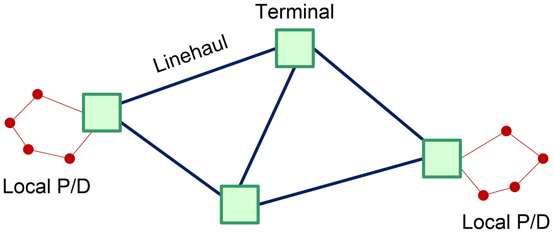
Less-than-truckload (LTL) trucking combines several of these alternatives in the terminal network of Fig. 2, repeated from Lecture 3.2, Sec. 1.2:
Figure 2: The logistics network used for less-than-truckload (LTL) and package express (PX). Local pickup and delivery (P/D) at each end, linehaul between terminals.
LTL is a mix of the alternatives. From the customers to the origin terminal it is collecting: a truck visits the customers, picks up their freight and takes it to the terminal. From terminal to terminal the transport is point to point, typically on a much bigger truck, and a terminal facility is basically just a big cement floor, where freight is offloaded and pieces of it go to other trucks going in other directions, so that the linehaul really is a network, and the freight ultimately ends up at its destination terminal. Delivery from there is peddling: the truck is loaded up and, as with the Amazon delivery, makes multiple stops. A carrier’s truck can seem never really empty, with always something to be delivered or something picked up, so that all of its stops would have to be considered together; but a vehicle can make several routes during one day, with periods in between when it is essentially empty, and breaking its work into pieces at those periods simplifies the analysis. If ten items are picked up, three of them delivered and then five more picked up, the truck is never empty and the stops are one route; if everything picked up has been dropped off and the truck is empty again, what follows is taken as a separate route. The TSP, the way it is treated here, only works for two of these situations, peddling and collecting. It cannot handle any of the alternatives that mix pickups and deliveries, which need more complicated ways of doing things to enforce the sequencing, the subject of Lecture 5.2. What makes the TSP easy is that everything is loaded at one point and all that has to be figured out is the sequence in which to make the deliveries, or, the opposite, all that has to be determined is where to make the pickups, with everything then taken to a single drop-off. That is a much easier problem than loading freight and then making deliveries and other pickups along the way.
The problem is to find a connected sequence through all nodes of a graph that minimizes total arc cost. The sequence is termed a tour since it returns to its starting node, and finding one is a subroutine in most vehicle routing problems. A node sequence can represent a route only if all pickups and/or deliveries occur at a single node, the depot of Fig. 3. A node sequence is a permutation followed by its start node, as in Table 1.
Show the code that draws this figure
# Code block 2: the six-node tour, each arc from the node it leavesP6 = [0.00.0; 0.01.2; 0.852.0; 1.71.2; 1.70.0; 0.85-0.8] # nodesr6 =0.16# node radius, data unitstour = [1, 2, 3, 4, 5, 6, 1]fig =Figure(size = (300, 300))ax =Axis(fig[1, 1]; aspect =DataAspect())hidedecorations!(ax); hidespines!(ax)for k in1:length(tour)-1# each arc, outline to outline p, q = P6[tour[k], :], P6[tour[k+1], :] u = (q .- p) ./hypot((q .- p)...) t, h = p .+ r6 .* u, q .- r6 .* uarrows2d!(ax, [t[1]], [t[2]], [h[1] - t[1]], [h[2] - t[2]]; color = ink, shaftwidth =1.4, tipwidth =9, tiplength =9)endfor i in1:size(P6, 1) # nodes over the arcs dep = i == tour[1] # the depot, in redpoly!(ax, Circle(Point2f(P6[i, 1], P6[i, 2]), r6); color =:white, strokecolor = dep ? redc : bluec, strokewidth = dep ? 2.4:1.6)text!(ax, P6[i, 1], P6[i, 2]; text =string(i), color = ink, fontsize =13, align = (:center, :center))endtext!(ax, -0.25, 0.0; text ="Depot", color = redc, fontsize =13, align = (:right, :center))xlims!(ax, -1.0, 2.1); ylims!(ax, -1.1, 2.3)fig
Figure 3: A tour of six nodes, starting and ending at the depot, node 1.
Table 1: The tour of Fig. 3 as a node sequence \pi: each position k in the sequence, above, and the node \pi_k visited there, below. Positions 1 to 6 are a permutation of the six nodes, and position 7 is its start node again.
\boldsymbol{k}
1
2
3
4
5
6
7
\pi_k
1
2
3
4
5
6
1
For the six nodes of Fig. 3, the number of possible tours is
n = 6 \Rightarrow ( n - 1 ) ! = 120 \text{ possible solutions}
\tag{1}
where
n
=number of nodes, the depot included.
The count is the factorial of n - 1, rather than of n, because the starting node of a route is arbitrary.
Few students reach this point in operations research or engineering without having seen the TSP in several classes, since it is a piece of a lot of things. The problem is to find a connected sequence of points that minimizes total cost, and the sequence is called a tour when it starts and ends at a depot, typically a distribution center. In a peddling situation, the vehicle is loaded at the depot and makes all of its drop-offs, the last of them at node 6 of Fig. 3. The vehicle is then empty, but by convention the TSP includes the cost of getting back to the depot, so a tour is a route plus the return to the depot. The convention could be dropped, and it would be perfectly fine to assume the route ends at node 6, so it is not an assumption that is important to what is being done; it can be made or not. As a result, a tour can be represented just by the sequence of node locations, starting at the depot, visiting the others in order and ending at the depot again. Mixing pickups and deliveries is more difficult because the sequence carries no information about which stops are pickups and which are deliveries; here the stops are taken to be all pickups or all deliveries, and all that matters is the sequence of the locations. The tour is effectively a permutation of the integers 1 through 6, with its first value, here 1, repeated at the end to model the return, so a tour of n nodes is a sequence of length n + 1. With n = 6 there are (n - 1)! = 120 possible tours (Eq. 1), and with today’s computers it would be easy to look at all of them, so brute force is reasonable for six nodes. TSPs in logistics with n equal to a thousand are probably not seen very much, but 100 to 200 nodes is definitely within the ballpark, and at n = 100 the number of tours is far too large for brute force.
A delivery van’s day is a TSP of that size. The 6,112 Amazon routes in the training data of the 2021 Amazon Last Mile Routing Research Challenge averaged 148 stops, with a tenth of them at 105 stops or fewer and a tenth at 186 or more, over an average route time of 8.1 hours, 4.5 of them spent serving the stops.1
The TSP is the basic routing problem, and in vehicle routing problems it is basically just a subroutine. What makes it simple and easy to solve is that it is unconstrained: any permutation is a feasible route. All that is done is to take a permutation of the integers 1 through 6 and make it into a tour, assuming a return to wherever it starts, by repeating its first node, the depot 1, at the end. The tour can also be thought of in arcs rather than nodes, and that is the better way, since it is how the problem is formulated, in Sec. 2, and how a tour is changed, by moving arcs around, in Sec. 3.
Location sequence, not route. A TSP’s tour is a location sequence, the order in which its nodes are visited. Route is kept for the pickup and delivery routes of Lecture 5.2, whose shipments each have their own origin and destination.
A tour’s sequence of nodes is called a location sequence rather than a route, although route might seem the more appropriate term. The reason is that the pickup and delivery routes of Lecture 5.2, whose shipments each have their own origin and destination, distinguish a route from a location sequence, and the two are not the same thing; so for the TSP the term is location sequence, for consistency with that later discussion. The cost of a tour is then the sum of the costs of the segments of its location sequence.
When the arc costs are asymmetric, there are only best-known solutions for large n, among the (n - 1)! tours of Eq. 2. When they are symmetric, c_{ij} = c_{ji}, the count is halved (Eq. 3), and the TSP is solved to optimality using binary integer programming (BIP), the subject of Sec. 2. In the Euclidean case, the arc costs are the distances between nodes, as in Fig. 4.
For an asymmetric and a symmetric TSP, the counts of tours are
\hphantom{\underset{\displaystyle \text{Symmetric:}}{\text{Asymmetric:}}}\mathllap{\text{Asymmetric:}}\quad \hphantom{\underset{\displaystyle \text{solutions}}{\text{solutions}}}\mathllap{\text{solutions}} = \mathrlap{( n - 1 ) ! \qquad n = 13 \Rightarrow \approx \frac{1}{2} \text{ billion}}\hphantom{\underset{\displaystyle \frac{( n - 1 ) !}{2} \qquad c_{ij} = c_{ji}}{( n - 1 ) ! \qquad n = 13 \Rightarrow \approx \frac{1}{2} \text{ billion}}} \tag{2}
\hphantom{\underset{\displaystyle \text{Symmetric:}}{\text{Asymmetric:}}}\mathllap{\text{Symmetric:}}\quad \hphantom{\underset{\displaystyle \text{solutions}}{\text{solutions}}}\mathllap{\text{solutions}} = \mathrlap{\frac{( n - 1 ) !}{2} \qquad c_{ij} = c_{ji}}\hphantom{\underset{\displaystyle \frac{( n - 1 ) !}{2} \qquad c_{ij} = c_{ji}}{( n - 1 ) ! \qquad n = 13 \Rightarrow \approx \frac{1}{2} \text{ billion}}} \tag{3}
where
c_{ij}
=cost of the arc from node i to node j.
Show the code that draws this figure
# Code block 3: a tour with crossing arcs, and the arcs that uncross itPX = [0.00.0; 0.740.73; 1.790.73; 2.530.0; 1.79-0.74; 0.74-0.74]rx =0.13# node radius, data unitscrossing = [6, 1, 2, 5, 4, 3, 6] # arcs 2→5 and 3→6 crossuncrossed = [(2, 3), (3, 4), (4, 5), (5, 6)] # 2→3, segment 3-4-5, 5→6functionarc!(ax, i, j; color = ink, dashed =false, off =0.0) p, q = PX[i, :], PX[j, :] u = (q .- p) ./hypot((q .- p)...) v = [u[2], -u[1]] .* off # shifted off the black arc t, h = p .+ rx .* u .+ v, q .- rx .* u .+ vif dashed # a dashed shaft, then its headlines!(ax, [t[1], h[1] -0.06u[1]], [t[2], h[2] -0.06u[2]]; color = color, linewidth =1.2, linestyle =:dash)scatter!(ax, [h[1] -0.04u[1]], [h[2] -0.04u[2]]; marker =:rtriangle, rotation =atan(u[2], u[1]), markersize =8, color = color)elsearrows2d!(ax, [t[1]], [t[2]], [h[1] - t[1]], [h[2] - t[2]]; color = color, shaftwidth =1.3, tipwidth =8, tiplength =8)endendfig =Figure(size = (300, 210))ax =Axis(fig[1, 1]; aspect =DataAspect())hidedecorations!(ax); hidespines!(ax)for k in1:length(crossing)-1arc!(ax, crossing[k], crossing[k+1])endfor (i, j) in uncrossed # beside 4→3 and 5→4, offsetarc!(ax, i, j; color = redc, dashed =true, off = i ==2|| i ==5 ? 0.0:-0.07)endfor i in1:size(PX, 1) # nodes over the arcspoly!(ax, Circle(Point2f(PX[i, 1], PX[i, 2]), rx); color =:white, strokecolor = bluec, strokewidth =1.6)endxlims!(ax, -0.3, 2.85); ylims!(ax, -1.0, 1.0)fig
Figure 4: A tour whose arcs cross (black), and the arcs that replace the crossing pair (red, dashed), traveling the segment between them the other way.
Even a problem with n = 13 already has about half a billion solutions (Eq. 2), so no direct approach that looks at all of them is feasible. The reason for n - 1 instead of n is that the starting node is arbitrary: node 1 or any of the others could be picked to start, so n! can be divided by n, leaving (n - 1)!. Where the distances are symmetric, the count reduces to (n - 1)!/2 (Eq. 3). Finally, where the arcs are Euclidean, the distances modeled as Euclidean or great circle distances between points, there is a nice heuristic for looking at routing solutions in many situations: whenever a route has two arcs crossing each other, as in Fig. 4, it cannot be optimal. It can always be improved by getting rid of the crossover.
The TSP is stated as a model in Model 1. Its mathematical formulation, Eq. 4, takes the cheapest of the (n - 1)! tours of Eq. 1, each a permutation of the nodes other than the depot. Ex. 1 does exactly that for ten cities, by brute force. Sec. 2 formulates it as a math program, a restriction of the linear assignment problem, Model 1 in Lecture 4.2, with one constraint added, and Sec. 3 solves it by improving a tour, searching the permutations one change at a time.
minimize: total cost of a tour through every node
solve for:
(a) tour, a sequence that visits each node exactly once and returns to its starting node.
subject to:
(a) Leave: each node is left exactly once;
(b) Enter: each node is entered exactly once; (c) Single tour: the arcs used form one connected cycle through all the nodes, not several.
assumptions:
(a) arc costs are given and need not be symmetric;
(b) cost of a tour is the sum of the costs of its arcs, including the return to the start.
=tour, the route as a sequence of nodes (\pi_1, \ldots, \pi_{n+1}) of Table 1, starting and ending at the depot, node 1
\Pi(S)
=permutations of the set S.
One of the goals of doing a mathematical formulation, as opposed to a math-programming formulation, is that, in the math formulation, it is typically obvious what the brute force needs to be. The fact that one is minimizing over all permutations in the math formulation provides an obvious way to do the brute force. The basic idea is to do brute-force optimization as the initial approach to get insight and get a known optimal solution, which other heuristic or math programming techniques can be judged against.
Combinatorial optimization refers to procedures used to find solutions from a collection of finite objects that characterize possible solution instances. These procedures fall into three broad categories. Brute-force optimization is to enumerate all possible solutions to find the global optimum. Heuristics look at a small fraction of possible solutions to find a local optimum that may not be the global optimum. Optimal procedures look at a small fraction of possible solutions to find the global optimum solution.
Heuristics and optimal procedures efficiently look at a small fraction of the possible solution instances to find a locally or globally optimal solution, but it is possible in many cases if the number of solutions is not too big to brute-force generate all possible solutions to find the global optimum. The ability to generate solution instances is useful for many reasons. One is brute-force optimization: if “small enough” (around n = 12, typically), it can be used to find the global optimum by searching through all instances. Each candidate solution can be evaluated directly by a rule, algorithm, or simulation that would be difficult or impossible to express in the precise mathematical form needed for traditional optimization. Another is heuristic validation: test heuristics on small instances where the global optimum can be determined in order to validate before using the heuristic for larger instances where it is not feasible to generate all instances.
Beyond some size, any combinatorial problem has many more potential solutions than there would ever be room or time to evaluate, so brute force always hits some upper limit. It is still worth the time, because computers are now so fast and have so much storage space that what would have been completely infeasible for even the smallest problems 20 years ago is now within the realm of the reasonable. Where there is no other way of getting an idea of how to solve a problem, a brute-force approach might be the only one that is actually feasible.
A brute-force version of at least a small version of a problem can be up and running in minutes, or at most an hour or so. Once it is, there is a validated solution to the problem, and for many problems it is hard even to come up with a valid solution once they get complicated enough, beyond n equal to 1, 2 or 3. That solution can then be used to validate heuristic solutions, and even math-programming formulations, confirming that on the smaller problems the math program gives the same correct optimal answer.
Example 1: Ten NC cities by brute force
Determine the minimum great circle distance tour through the ten NC cities with a population over 100,000 of Ex. 2 in Lecture 4.1 by brute force, looking at every tour of the mathematical formulation Eq. 4.
Code block 4 reads the ten cities from the Logjam gazetteer, as Ex. 2 in Lecture 4.1 does:
# Code block 4: the NC cities over 100,000, from the Logjam gazetteerusingDataFrames, Logjamdf =filter(r -> (r.STFIP ==st2fips(:NC)) && (r.POP >100_000),usplace())select!(df, :NAME, :LAT, :LON, :POP)prt(df)
NAME LAT LON POP
───────────────────────────────────────
Cary 35.78 -78.82 174,721
Charlotte 35.21 -80.83 874,579
Concord 35.39 -80.64 105,240
Durham 35.98 -78.90 283,506
Fayetteville 35.08 -78.97 208,501
Greensboro 36.10 -79.83 299,035
High Point 35.99 -79.99 114,059
Raleigh 35.83 -78.64 467,665
Wilmington 34.21 -77.89 115,451
Winston-Salem 36.10 -80.26 249,545
One permutation at a time. As long as the permutations are not all generated first, brute force stays feasible even for fairly large problems: each call for a permutation gives just the next one in the sequence, not all of the billions or trillions of them. It may take some time, but it uses essentially no memory, since none of those permutations has to be stored. The Combinatorics package’s permutations is designed to generate one at a time, which is what makes this convenient.
Code block 5 computes the great circle distances between them, the arc costs c_{ij} of a symmetric TSP, and computes the cost of every tour that starts and ends at the first city, as the permutations of cities 2 to 10 taken one at a time, keeping the cheapest, which is the mathematical formulation of Eq. 4 worked in full:
# Code block 5: great circle distances, and every tour by brute forceusingCombinatoricsP =hcat(df.LON, df.LAT) # one row per cityD =dists(P, P, :mi)n =size(D, 1)tours = ([1; p; 1] for p ∈permutations(2:n))TCᵒ, πᵒ =minimum((sum(D[π[k], π[k+1]] for k ∈1:n), π)forπ∈ tours)@showlength(tours) # the tours looked at@show TCᵒ # the cheapest of them@show πᵒ; # the tour that costs it
1
Parentheses, not square brackets, make tours a generator: each tour is built from the next permutation only when minimum asks for it, so the tours are looked at one at a time and never held in memory together. Square brackets would build and store every tour first.
2
Each tour is paired with its cost, the sum of Eq. 4, and minimum compares the pairs by cost first, so it returns the cheapest cost together with its tour.
With n = 10, the 362,880 tours looked at are the (n - 1)! of Eq. 1, and the cheapest costs 487.69 mi. Its reverse costs the same, since great circle distances are symmetric, which is why Eq. 3 halves the count.
The optimal tour of the ten cities is 1-4-6-7-10-3-2-5-9-8-1, of 487.69 mi, the cheapest of all 362,880 tours.
2. TSP as a MILP
Solved exactly, as a binary integer program (BIP; Lecture 2.7, Sec. 1), the TSP has a formulation that has an exponential number of constraints to eliminate subtours, which calls for constraint generation techniques.
The TSP solved as a binary integer program has one difficulty. Its obvious formulation, here the linear assignment problem of Lecture 4.2, is an easy problem to solve, but its solutions can have what are called subtours, and they are feasible for it. With six nodes, for example, a solution could be two separate subtours instead of one route that visits all of the nodes and returns to its start, and that is obviously not a solution of the TSP. Over 40 or 50 years of integer programming, the only way found to get rid of subtours is to add constraints that make them infeasible: given a solution like that, a constraint is added that forces its nodes to be joined into one route. There is an exponential number of those constraints, one for each subset of the nodes, so handling all of the possibilities at once would run out of space for any but a small problem, which is not feasible. When a problem does need to be solved as a binary integer program, most commercial solvers, such as Gurobi or CPLEX, add constraints while the problem is being solved: at a node of the branch-and-bound tree, only the constraints needed for the partial solution seen at that point are added, on an as-needed basis, and that makes the problem feasible to solve from the point of view of memory. This is how a TSP solution is verified to be optimal: the TSP is solved as a binary integer program until it reaches a final solution, which is then guaranteed to be optimal. A solution from a heuristic procedure can never be guaranteed optimal without doing that; it is just the best known.
Math programming researchers have been all over the TSP, a great problem for developing new techniques. From a practical point of view, a math program is never really needed for a problem that truly is just a TSP, but because the TSP is a simplified version of harder problems, many of the techniques developed on it are useful for more complex ones: it is a testing ground for math programming, binary integer programming among them. Probably the most common technique is to add constraints that keep subtours from forming. The hardest thing in modeling the TSP as a math program is to keep out solutions in which the vehicle starts from a node and returns to it without visiting all of the stops, which is a subtour, so additional constraints are needed that keep the vehicle from coming back too soon and force it to visit all of the nodes. That requires an exponential number of constraints, on the order of 2^n, far more for n = 100 than a computer has storage for. In practice a constraint is added only when it is needed to eliminate a subtour found in the solution so far, rather than enumerating every possible subtour constraint, and that gives a pretty effective procedure.
This can be done with any solver, open-source or commercial, one round at a time: solve, add the constraints the solution violates, and solve again. That is how this section’s implementation of Model 1 does it with HiGHS, the open-source solver of this course (Table 2 in Lecture 2.7). Some solvers, among them the commercial Gurobi and CPLEX, can also add the constraints during a single solve, at the nodes of the branch-and-bound tree.
NoteOther formulations of the TSP
The online database of TSPs that were really challenging in the 1980s, problems of about 100 nodes taken from real problems such as tours of locations in Berlin, had all been solved to optimality by the 1990s, and today a problem has to be far larger than anything logistics engineering is concerned with before current techniques cannot solve it. Another formulation, developed very early, in 1960, has only a quadratic number of constraints, on the order of n^2, which is achievable, and with it no constraints have to be added as needed. Its problem is that, like the weak formulation of the uncapacitated facility location (UFL) problem in Lecture 2.7, Sec. 2, it is very weak: solved as a linear program, its solution is far from the optimal integer solution, so a problem of n = 100 might run for a day where the strong formulation, with its constraints added as needed, might solve in minutes. It is a choice of difficulty: the constraints added as needed, with a tight formulation, or a quadratic number of constraints and a problem that takes forever to solve. All of that is literally academic, since the TSP never really needs a math program, but it is good to have that perspective.
The 1960 formulation is that of Miller, Tucker and Zemlin.2 It is known by their initials as MTZ.
The database is TSPLIB, whose instances include a tour of 52 locations in Berlin.3
The math-programming formulation of Model 1 is on a complete graph G = (V, A) on n nodes:
=\begin{cases} 1, & \text{if the tour goes from node } i \text{ directly to node } j \\ 0, & \text{otherwise} \end{cases}
V
=nodes
=\{1,\dots,n\}
A
=arcs
=\{(i,j) : i,j = 1,\dots,n\}
c_{ij}
=cost of each arc (i,j) (cost) c_{ii} = \infty
S
=subset of the nodes, neither empty nor all of them
|S|
=number of nodes in S.
Rows (a) and (b) of Eq. 5 are Model 1’s degree constraints, leave and enter, and row (c) is its subtour elimination constraint, single tour. A subtour through the nodes of a subset S would use |S| arcs among them, and row (c) allows at most |S| - 1, so no subtour can form. Without the subtour elimination constraint, the TSP relaxes to the LAP, the linear assignment problem of Lecture 4.2, with every node both a supply node and a demand node. The TSP is symmetric if c_{ij} = c_{ji}, and Euclidean if the c_{ij} are Euclidean distances.
The implementation of the formulation below starts from rows (a) and (b) alone, which are the assignment problem, and solves it. It then finds the subtours in the solution, adds row (c) for each of them, and solves again, until the solution is a single tour; each pass is a round, and the rounds are returned with the tour so that they can be looked at. Adding only the constraints that a solution violates is the constraint generation described above, done one round at a time rather than inside the branch-and-bound tree.
Model 1 implementation: Math-programming formulation
# Model: traveling salesman problemusingJuMP, HiGHSfunctionsubtours(succ) # the cycles of a successor vector S, seen =Vector{Vector{Int}}(), falses(length(succ))for k ∈eachindex(succ) seen[k] &&continue Sₖ, i =Int[], kwhile !seen[i] # follow the arcs back to k seen[i] =truepush!(Sₖ, i) i = succ[i]endpush!(S, Sₖ)endreturn SendfunctionTSP(c)size(c, 1) ==size(c, 2) ||# assumption (a): each pair's costerror("arc costs must be a square matrix") V =1:size(c, 1) model =Model(HiGHS.Optimizer)@variable(model, x[i ∈ V, j ∈ V; i ≠ j], Bin) # no arc i to i@objective(model, Min,sum(c[i, j] * x[i, j] for i ∈ V, j ∈ V if i ≠ j))@constraint(model, leave[i ∈ V],sum(x[i, j] for j ∈ V if j ≠ i) ==1) # (a)@constraint(model, enter[j ∈ V],sum(x[i, j] for i ∈ V if i ≠ j) ==1) # (b)set_silent(model)set_attribute(model, "mip_rel_gap", 0.0) rounds = []whiletrueoptimize!(model)termination_status(model) == JuMP.OPTIMAL ||error(termination_status(model)) succ = [findfirst(j -> j ≠ i &&value(x[i, j]) >0.5, V) for i ∈ V] # the node after each node S =subtours(succ)push!(rounds, (TC =objective_value(model), S = S))iflength(S) ==1# a single tour: donereturn (TC =objective_value(model), tour = [S[1]; S[1][1]], rounds = rounds)endfor Sₖ ∈ S # (c), for each subtour found@constraint(model,sum(x[i, j] for i ∈ Sₖ, j ∈ Sₖ if i ≠ j) ≤length(Sₖ) -1, base_name ="singletour")endendend
1
HiGHS stops by default once its solution is proved within 0.01% of the optimum; a gap of 0 makes it prove the tour optimal, which the Landmark checks of Ex. 2, 3 and 4 rely on.
2
A solved binary can come back as 0.9999999 rather than 1, so a value above 0.5 is read as 1; each node’s successor is the one node its row of x sends it to.
3
A subtour through the nodes of S_k uses |S_k| arcs among them, and a tour can use at most |S_k| - 1, so the subtour just found cannot come back; others can, which is why the loop solves again.
TSP (generic function with 1 method)
Example 2: Ten NC cities as a MILP
Determine the minimum great circle distance tour through the ten NC cities of Ex. 1, by solving the formulation of Model 1 one round at a time, starting from its assignment problem, and determine whether its tour is the one Ex. 1 found by brute force.
Code block 6 solves Model 1 on the great circle distances of Code block 5, printing the cost and the number of subtours of each round:
# Code block 6: the TSP solved in roundsnc10 =TSP(D)rounds =DataFrame(round =eachindex(nc10.rounds), mi = [rd.TC for rd in nc10.rounds], subtours = [length(rd.S) for rd in nc10.rounds])prt(rounds)
Round 1 solves rows (a) and (b) alone, the assignment problem. Its solution, 301.99 mi, leaves and enters each city exactly once, as the two rows require, and is still not a tour: it is 4 subtours, Cary, Durham and Raleigh; Charlotte and Concord; Fayetteville and Wilmington; and Greensboro, High Point and Winston-Salem (Fig. 5). Adding row (c) for each of them and solving again joins them into 3 larger subtours, at 450.86 mi, and adding row (c) for those gives, in round 3, a single tour of 487.69 mi. Each round solves the TSP with only some of its subtour constraints, so its cost is a lower bound on the optimal tour’s, the Bounds check of Lecture 1.2, and the costs can only rise from round to round; the tour of the last round satisfies every subtour constraint without their having been added, so it is the optimal tour. It is also the tour Ex. 1 found by brute force, at the same 487.69 mi, so the optimum known before the math program was solved is a Landmark check of Lecture 1.2 on it, confirming that on this small problem the formulation and its implementation give the correct optimal answer.
Show the code that draws this figure
# Code block 7: each round's solution, drawn on a map# (makemap draws one map per figure, so the three frames are plain axes in# longitude and latitude, scaled by the cosine of the mean latitude)(xl, yl) =mapbbox(df.LON, df.LAT; xexpand =0.14, yexpand =0.16)lab =Dict(aligntext(df.LON, df.LAT; offsetamt =5))al, os =copy(lab[:align]), copy(lab[:offset])# moved by hand where, in some round, an arc, the border or another name# crosses the place Logjam's aligntext givesfor (nm, a, o) in [("Charlotte", (:right, :bottom), (-5, 3)), ("Concord", (:left, :top), (5, -3)), ("High Point", (:left, :top), (4, -4)), ("Durham", (:left, :bottom), (5, 3)), ("Cary", (:right, :top), (-6, -4)), ("Fayetteville", (:right, :top), (-4, -4)), ("Wilmington", (:right, :top), (-3, -4))] i =findfirst(==(nm), df.NAME) al[i], os[i] = a, oendfig =Figure(size = (687, 640))cells = [fig[1, 1], fig[1, 2], fig[2, 1:2]]for (k, rd) inenumerate(nc10.rounds) nS =length(rd.S) ax =Axis(cells[k]; autolimitaspect =1/cosd(sum(yl) /2), title ="Round $k: $(round(rd.TC, digits =2)) mi, "* (nS ==1 ? "one tour":"$nS subtours"), titlesize =13, titlefont =:regular)hidedecorations!(ax); hidespines!(ax)limits!(ax, xl[1] -0.3, xl[2] +0.3, yl...) # room for the nameslines!(ax, Logjam.usstates()...; color = (bluec, 0.6), linewidth =0.75)for Sₖ in rd.S, (a, b) inzip(Sₖ, circshift(Sₖ, -1))lines!(ax, [df.LON[a], df.LON[b]], [df.LAT[a], df.LAT[b]]; color = redc, linewidth =1.6)endscatter!(ax, df.LON, df.LAT; color = bluec, markersize =8)text!(ax, df.LON, df.LAT; text = df.NAME, fontsize = k <3 ? 11:12, color = ink, align = al, offset = os)endrowsize!(fig.layout, 2, Relative(0.6))fig
Figure 5: The three rounds of Ex. 2: the assignment problem’s four subtours, then three, then the optimal tour.
The optimal tour of the ten cities is 487.69 mi, found in round 3.
3. Two-opt improvement
In practice the TSP is solved by a mix of construction and improvement procedures, the split of Lecture 2.4, Sec. 3.
The same theme was seen with the UFL problem of Lecture 2.4: its ADD procedure constructs a solution, its DROP procedure is another way of constructing one, starting from the other end, and its exchange procedure, EXCHG, is the improvement side. A heuristic for the TSP is likewise some mix of construction and improvement procedures.
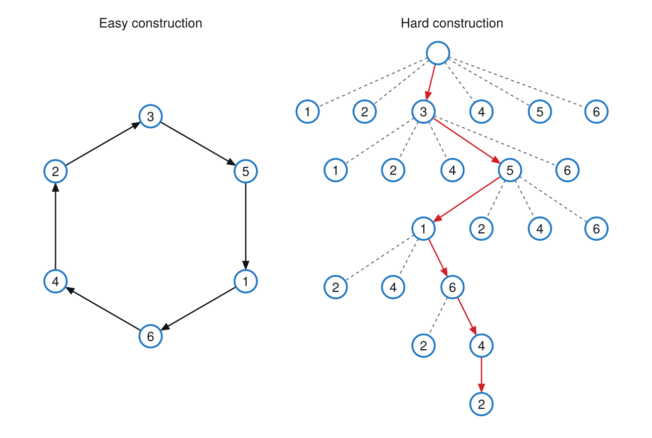
For the TSP, construction is easy since any permutation is feasible and can then be improved, as Fig. 6, repeated from Lecture 2.4, shows on six stops. Lecture 2.4’s two kinds of construction separate the TSP from the VRP of Lecture 5.3. Under easy construction (e.g., the quadratic assignment problem and the TSP), the lack of constraints makes any random point or permutation a feasible solution, and it can then be improved, allowing construct-then-improve multiple times, or what is termed multi-start. Under hard construction (e.g., bin packing and the VRP), there is almost no chance of generating a random feasible solution due to constraints on what is a feasible solution, so there is a need to include randomness as a solution is generated in order to construct multiple different solutions (which “might” then be able to be improved).
Figure 6: Two ways to construct a tour of six stops. Under easy construction any random permutation is already a tour, so one is generated and then improved. Under hard construction the tour is built one decision at a time, each step checked for feasibility, with the chosen path in red. Here both routes arrive at the same tour.
The tree of Fig. 6 counts the tours as well. Any of the nodes could be picked as the starting node; arbitrarily picking node 3 eliminates one degree of freedom, and there are then five choices for the second node, four for the third, then three, two and one. Once every node but node 2 has been placed, there is no decision left, and node 2 has to be the last.
NoteSpacefilling curve
A spacefilling curve is a construction procedure for the TSP that needs no cost matrix: it uses only the XY locations of the points. A cost matrix is needed only to determine the cost of the tour it gives.
The tour’s sequence is determined by sorting each point’s position along a 1-D line covering the 2-D space, the curve of Fig. 7.4 The four points of the figure are at positions 2: 0.021, 3: 0.154, 1: 0.471 and 4: 0.783, so sorting them gives the sequence 2, 3, 1, 4, or 1, 4, 2, 3 as a tour that starts at point 1.
The spacefilling curve is a technique for constructing a TSP solution, kept here at first for historical reasons, but it has quite a lot of relevance today. It was developed by John Bartholdi of Georgia Tech, whose campus buses appear in Lecture 1.3: each bus is held at a stop to keep a constant headway, which avoids bunching and lowers the average waiting time, again a very low-tech solution. A spacefilling curve is a one-dimensional curve that fills a two-dimensional space. In Fig. 7 it starts at the corner (0, 0) and ends back right next to it, like a long string spread out until it covers the square, and the points along it are numbered from 0 at its start to 1 at its end. For a TSP, those numbers are laid over a map. Bartholdi developed the idea for Meals on Wheels in Atlanta, before there were PCs: each stop where food was to be delivered was given the number of its point on the curve, written on an index card, so that one house might be at 0.471 and others at 0.021, 0.154 and 0.783. The only computation was sorting the cards. The planner sorted the day’s cards, perhaps 200 of them, into order by their numbers, which took five or ten minutes, and handed out the sorted stack in order, the first run of cards to the first driver, the next run to the second, and so on. It is a robust procedure, since a dropped stack can be put back in order by its numbers, and a perfectly good routing solution, though not an optimal one. Its application in logistics is now obsolete. Its application elsewhere is not: when Bartholdi was the external reviewer of NC State’s operations research program, around 2016 or 2017, he reported that the 1988 paper was being cited quite a bit, because of geographic mapping applications and machine learning. A database of two-dimensional geographic information has no single key, since x and y have no obvious order, and a spacefilling curve gives each point one, which allows a join of two spatial databases. The curve has been more popular than ever.
The Meals on Wheels system was published in 1983. Its meals were delivered by four paid, part-time drivers, each delivering 40 to 50 meals to 30 to 40 locations between 10 a.m. and 2 p.m.5
The implementation of the spacefilling curve has two functions. The first, sfcpos, finds the position of a point of the unit square along the curve by determining which of four quadrants it is in and then, recursively, where it is within that quadrant, to a depth of k binary digits; the second, tspspfillcur, scales the points to the unit square and sorts them by position.
Model 1 implementation: Spacefilling curve construction
# Model: traveling salesman problem, spacefilling curve construction# Position θ in [0, 1) of the point (x, y) of the unit square along# the spacefilling curve, using k binary digits of x and yfunctionsfcpos(x, y, k =8)if k ==0return0.5# center of the last squareend VN = [01; 32] # order the quadrants are visited q = VN[min(floor(Int, 2x +1), 2), min(floor(Int, 2y +1), 2)] s =sfcpos(2abs(x -0.5), 2abs(y -0.5), k -1) # within qif q ==1|| q ==3 s =1- s # quadrants 1 and 3 run backwardend θ = (q + s -0.5) /4return θ -floor(θ)end# Tour of the points in the rows of XY in the order of their positions# along the spacefilling curve, starting and ending at point 1functiontspspfillcur(XY, k =8) x = XY[:, 1] y = XY[:, 2]ifany(XY .<0) ||any(XY .>1) # scale to the unit square, w =max(maximum(x) -minimum(x), maximum(y) -minimum(y)) x = (x .-minimum(x)) ./ w # keeping the aspect ratio y = (y .-minimum(y)) ./ wend θ =sfcpos.(x, y, k) loc =sortperm(θ) # points in curve order i1 =findfirst(loc .==1)return [loc[i1:end]; loc[1:i1-1]; 1]end
tspspfillcur (generic function with 2 methods)
Code block 8 computes the positions of the four points of Fig. 7 and their tour, and Code block 9 the positions of an 11 × 11 grid of points of the unit square, which can be read against Fig. 7:
# Code block 8: the four points, their positions and their tourXY4 = [0.80.8; 0.10.2; 0.30.7; 0.70.2] # points 1 to 4θ4=sfcpos.(XY4[:, 1], XY4[:, 2])@showround.(θ4, digits =3)@showtspspfillcur(XY4);
# Code block 9: positions on a grid, rows from y = 1 down to y = 0g = (0:10) ./10Θ = [sfcpos(x, y) for y inreverse(g), x in g]prt(round.(Θ, RoundNearestTiesAway, digits =3); rows =string.(reverse(g)), cols =string.(g), row_title ="y", allfrac =3)
# Code block 10: the curve, by joining a grid's points in curve ordergr =0:0.02:1X = [x for y in gr, x in gr]Y = [y for y in gr, x in gr]ij =sortperm(vec(sfcpos.(X, Y))) # the grid's points in curve orderfig =Figure(size = (360, 360))ax =Axis(fig[1, 1]; aspect =DataAspect(), xticks =0:0.2:1, yticks =0:0.2:1, xgridvisible =false, ygridvisible =false)lines!(ax, vec(X)[ij], vec(Y)[ij]; color = (ink, 0.55), linewidth =0.5)# each label on a white card, centred beside its point and clear of the# tour (the axis is about 300 px across its 0 to 1)at = XY4 .+ [0.00.08; 0.10-0.07; -0.100.07; 0.10-0.07]scatter!(ax, at[:, 1], at[:, 2]; marker = Rect, color =:white, markersize =fill((76, 26), 4))r4 =tspspfillcur(XY4)lines!(ax, XY4[r4, 1], XY4[r4, 2]; color = bluec, linewidth =2)scatter!(ax, XY4[:, 1], XY4[:, 2]; color = redc, markersize =10)text!(ax, at[:, 1], at[:, 2]; text = [rich("$i: ", rich(string(round(θ4[i], digits =3)), color = bluec)) for i in1:4], color = ink, fontsize =13, align = (:center, :center))limits!(ax, 0, 1, 0, 1)fig
Figure 7: The spacefilling curve over the unit square, and the tour it gives through four points. Red is given: the points. Blue has to be determined: each point’s position along the curve, and the tour that sorting the positions gives.
On a problem whose optimal solution is known, the spacefilling curve does the worst, but it is arguably the easiest.
Ex. 4(c) measures its tour of the 100 NC counties against the optimal tour.
The one important thing about the TSP is how to improve a tour. A construction procedure is not really needed today: a randomly generated permutation of the integers is a feasible starting point, since any sequence of the numbers 1 through 6 is a valid tour, and it turns out that all of the work is done by the improvement procedure.
With maybe a hundred different random starting points, a solution probably within a percent of the optimal can be found, which Ex. 4 tests. The improvement procedure is two-opt (2-opt). Where the exchange procedure of the UFL in Lecture 2.4 exchanges nodes, 2-opt exchanges arcs. In Fig. 8, the letters a to f are the arcs of the tour 1-2-3-4-5-6-1, and the first change gets rid of arcs a and c and adds instead an arc from 1 to 3 and another from 2 to 4, replacing two arcs with two other arcs so that the tour is still feasible: it now goes from 1 to 3, back to 2 and over to 4. Since the two new arcs cross, that change does not improve the tour. Most changes do not, and 2-opt is looking for the few that do; with Euclidean costs a change that worsens the tour would show a crossing, and otherwise its cost would go up. Each change is so cheap to compute that the computer can be left to do the work, rather than designing something more specialized; unless there are thousands and thousands of nodes, a random permutation works fine, and that simplifies the effort quite a bit. A change is made by taking the segment between the two arcs removed and flipping it. Removing a and c flips 2-3 into 3-2; removing a and d gives the route 1-4-3-2-5, the segment 2-3-4 flipped; removing a and e flips everything from 2 to 5. These are the 2-opt changes, and they continue with b and d, b and e, and on through d and f. With n = 6 there are nine of them in all, n(n - 3)/2 (Eq. 6). That number grows as n^2, so even for n = 100, where looking at all of the tours is out of the question, the changes can be dealt with, and they give decent routes. This is worth spending some time to understand. Many arc changes are not feasible: any two arcs incident to the same node, such as a and f or a and b, cannot be exchanged, so two arcs can be exchanged only when at least one arc separates them.
Show the code that draws this figure
# Code block 11: the changes that remove arc a with arc c, and with arc d,# beside the table of all nine changestourarcs = [(1, 2, "a"), (2, 3, "b"), (3, 4, "c"), (4, 5, "d"), (5, 6, "e"), (6, 1, "f")] # 1-2-3-4-5-6-1, letteredfunctionarc6!(ax, i, j; color = ink, dashed =false, off =0.0) p, q = P6[i, :], P6[j, :] u = (q .- p) ./hypot((q .- p)...) v = [u[2], -u[1]] .* off # shifted to the arc's right t, h = p .+ r6 .* u .+ v, q .- r6 .* u .+ vif dashed # a dashed shaft, then its headlines!(ax, [t[1], h[1] -0.11u[1]], [t[2], h[2] -0.11u[2]]; color = color, linewidth =1.3, linestyle =:dash)scatter!(ax, [h[1] -0.09u[1]], [h[2] -0.09u[2]]; marker =:rtriangle, rotation =atan(u[2], u[1]), markersize =9, color = color)elsearrows2d!(ax, [t[1]], [t[2]], [h[1] - t[1]], [h[2] - t[2]]; color = color, shaftwidth =1.4, tipwidth =9, tiplength =9)endendmid(i, j) = (P6[i, :] .+ P6[j, :]) ./2fig =Figure(size = (687, 360))ax =Axis(fig[1, 1]; aspect =DataAspect())hidedecorations!(ax); hidespines!(ax)for (i, j, lab) in tourarcs # the tour, each arc letteredarc6!(ax, i, j) p, q = P6[i, :], P6[j, :] u = (q .- p) ./hypot((q .- p)...) m =mid(i, j) .-0.24.* [u[2], -u[1]] # outside the tourtext!(ax, m[1], m[2]; text = lab, color = dcc, fontsize =15, align = (:center, :center))endfor (i, j, off) in [(1, 3, 0.0), (3, 2, 0.07), (2, 4, 0.0)] # a with carc6!(ax, i, j; color = redc, dashed =true, off = off)endfor (i, j, off) in [(1, 4, 0.0), (4, 3, 0.07), (3, 2, -0.07), (2, 5, 0.0)] # a with darc6!(ax, i, j; color = bluec, dashed =true, off = off)endfor (i, j, c, dy) in [(1, 2, redc, -0.12), (1, 2, bluec, 0.12), (3, 4, redc, 0.0), (4, 5, bluec, 0.0)] # removed m =mid(i, j) # a mark on the arcscatter!(ax, [m[1]], [m[2] + dy]; marker ='×', markersize =22, color = c)endfor i in1:size(P6, 1) # nodes over the arcspoly!(ax, Circle(Point2f(P6[i, 1], P6[i, 2]), r6); color =:white, strokecolor = bluec, strokewidth =1.6)text!(ax, P6[i, 1], P6[i, 2]; text =string(i), color = ink, fontsize =13, align = (:center, :center))endxlims!(ax, -0.6, 2.3); ylims!(ax, -1.1, 2.3)# the table beside it: the arc letters over the tour, then each change of# the loop of Code block 12, its reversed segment boxedtb =Axis(fig[1, 2])hidedecorations!(tb); hidespines!(tb)text!(tb, (1:6) .+0.5, zeros(6); text =last.(tourarcs), color = dcc, font =:bold, fontsize =15, align = (:center, :center))text!(tb, 1:7, fill(-1.0, 7); text =string.(tour), color = ink, fontsize =14, align = (:center, :center))for y in (-0.5, -1.5) # the rules around the tourlines!(tb, [-0.7, 7.5], [y, y]; color = ink, linewidth =1.0)endchanges = [(i, j) for i =1:length(tour)-2 for j = i+2:min(length(tour)-1, length(tour)+i-3)]for (k, (i, j)) inenumerate(changes) y =-1.0- k πk =vcat(tour[1:i], reverse(tour[i+1:j]), tour[j+1:end])text!(tb, 0.0, y; text = tourarcs[i][3] *"-"* tourarcs[j][3], color = dcc, font =:bold, fontsize =14, align = (:center, :center))text!(tb, 1:7, fill(y, 7); text =string.(πk), color = ink, fontsize =14, align = (:center, :center)) c = k ==1 ? redc : k ==2 ? bluec : dcc # a-c and a-d as drawnlines!(tb, [i +0.6, j +0.4, j +0.4, i +0.6, i +0.6], [y -0.38, y -0.38, y +0.38, y +0.38, y -0.38]; color = c, linewidth =1.1, linestyle =:dash)endxlims!(tb, -0.8, 7.6); ylims!(tb, -10.6, 0.5)colsize!(fig.layout, 1, Aspect(1, 2.9/3.4)) # the tour at its aspectfig
Figure 8: Two 2-opt changes of the tour 1-2-3-4-5-6-1, whose arcs are lettered a to f, and all nine of its changes. Removing arcs a and c (red ×) adds the red arcs and reverses 2-3; removing arcs a and d (blue ×) adds the blue arcs and reverses 2-3-4. Each row of the table is the sequence a change gives, named by the two arcs it removes, with the segment it reverses boxed.
Code block 12 lists the nine changes of the tour 1-2-3-4-5-6-1, each with its segment flipped, in the order of the letters of Fig. 8, starting with a and c and ending with d and f:
# Code block 12: the nine 2-opt changes of the tour 1-2-3-4-5-6-1π= [1:6; 1]println(π)for i =1:length(π)-2for j = i+2:min(length(π)-1, length(π)+i-3)println(vcat(π[1:i], reverse(π[i+1:j]), π[j+1:end]))endend
1
j starts two past i, so the two arcs removed are never adjacent, and when i = 1 it stops one short, since the last arc, back into node 1, is adjacent to the first.
2
The tour up to \pi_i, then the segment from \pi_{i+1} to \pi_j reversed, then the rest: the arcs out of \pi_i and out of \pi_j are removed, and arcs from \pi_i to \pi_j and from \pi_{i+1} to \pi_{j+1} are added.
The number of sequences considered at the end to verify a local optimum, for n nodes, is the number of rows the loop of Code block 12 prints after its first:
\overbrace{\sum_{j = 3}^{n - 1} ( 1 )}^{\text{first arc } a} + \overbrace{\sum_{i = 2}^{n - 2} \sum_{j = i + 2}^{n} ( 1 )}^{\text{arcs } b \text{ to } n - 2} = \frac{n ( n - 3 )}{2} = 9 \text{ for } n = 6
\tag{6}
where
i
=position in the tour of the last node before the reversed segment
j
=position in the tour of the last node of the reversed segment.
It is a first improvement procedure: others look at all the possibilities and take the best, but this one makes any improvement as soon as it sees it, and the new sequence becomes the base point. Whenever there is an improvement, the clock is put back and the scan starts again at the first change; it is not a continuation.
The 2-opt procedure is a formulation of Model 1 written as pseudocode. Where Eq. 4 takes the minimum over every permutation, 2-opt looks only at the tours one change away from the current one, moves to the first of them that is cheaper, and stops at a tour that none of them improves. It is the loop of Code block 12 with a cost check added.6
Model 1 formulation: Two-opt improvement
algorithm twoopt;{ input: tour π = (π₁, …, πₙ₊₁) of n nodes, πₙ₊₁ = π₁; cost c(π) }{ output: tour πᵒ that no 2-opt change improves, and its cost TCᵒ }begin πᵒ := π, TCᵒ := c(π); { the start is the best so far } done := false; while not done do { until a scan improves nothing } begin done := true, i := 1; while done and i ≤ n − 1 do begin j := i + 2; while done and j ≤ min(n, n + i − 2) do begin π′ := π with πᵢ₊₁, …, πⱼ reversed; { a 2-opt change } if c(π′) < TCᵒ then { strictly better } πᵒ := π′, TCᵒ := c(π′), done := false; j := j + 1; end; i := i + 1; end; π := πᵒ; { scan again from the new tour } end; return πᵒ, TCᵒ;end;
Line 15 is the change of Fig. 8, the arcs from \pi_i and into \pi_{j+1} removed and the segment between them reversed, and line 16 keeps it only if it lowers the cost. The bounds on i and j in lines 10 and 13 are those of Code block 12, whose length(π) is n + 1, so that the two arcs removed are never adjacent, and they give the n(n - 3)/2 changes of Eq. 6. Line 17 sets done to false, which ends both scans at once, so the procedure takes the first improving change rather than the best one, and line 22 starts the scan again from the tour that change gave.
Model 1 implementation: Two-opt improvement
# Model: TSP, two-opt improvement# r: Initial route as a vector (can be TSP tour or shipment sequence).# rTCh: Function that calculates route cost: rTCh(route) -> cost.twoopt # (r, rTCh)
Steepest descent and first improvement are both improvement heuristic strategies used to refine a solution. Steepest descent thoroughly evaluates all neighboring solutions in each step and moves to the single best one, ensuring the greatest immediate gain but requiring more computation per iteration. In contrast, first improvement evaluates neighbors sequentially and selects the first one found that offers any improvement, making iterations faster but potentially taking smaller steps or settling into a less optimal local solution. In the TSP, neighbor evaluations (e.g., 2-opt changes) are cheap and improvements are frequent, so first improvement is preferred to explore more solutions in the same time.
A heuristic can itself be built from simpler heuristics. Multi-start is a meta-heuristic for the TSP, built from the implementations of two other heuristics, as the UFL hybrid of Lecture 2.4, Sec. 6, is built from three: it constructs a random tour, the easy construction of Fig. 6, improves it by 2-opt, and repeats from new random tours, keeping the best tour found.
Model 1 formulation: Multi-start
algorithm multistart;{ input: n nodes, cost c(π) of a tour π, number of starts N }{ output: best tour πᵒ found, and its cost TCᵒ }begin TCᵒ := ∞; for k := 1 to N do begin π := a random tour of the n nodes; { easy construction } π′, TC′ := twoopt with π; { improvement } if TC′ < TCᵒ then πᵒ := π′, TCᵒ := TC′; end; return πᵒ, TCᵒ;end;
Line 8 is the construction and line 9 the improvement; line 10 keeps the best tour over all of the starts, where 2-opt keeps the first improvement it sees.
Determine a tour of the six nodes of Fig. 3 by 2-opt improvement of the tour 1-2-3-4-5-6-1, under the arc costs D of Eq. 7, by hand, in Julia, and by multi-start from random starting tours, and determine how far the tours it finds are from the optimum.
From it, the procedure considers the nine changes of Code block 12 in order and keeps the first that lowers the cost; from the tour that gives, it starts its scan again. Table 2 lists every sequence it considers, in order, and Fig. 9 draws each tour it keeps, red given and blue to be determined:
Figure 9: The tours 2-opt keeps in Ex. 3(a), from the starting tour to the local optimum. Red is given: the cost of each arc. Blue has to be determined: the arcs each change adds, and the tour’s cost after it, with the cost before it in gray. The arcs a change removes are dashed and crossed (×).
Table 2: The sequences 2-opt considers in Ex. 3(a), in order, with their costs. In each, the segment its change reverses is shaded blue, and Change counts the changes looked at since the last tour kept, in the order of the rows of the table in Fig. 8; each kept sequence is the tour the scan starts again from. A scan stops at its first change that lowers the cost, so only the last, from the local optimum, looks at all 9 changes of Eq. 6, verifying that none is lower: 2-opt does its most work at the end.
Sequence
Cost
Change
1
1 2 3 4 5 6 1
38
start
2
1 3 2 4 5 6 1
39
1
3
1 4 3 2 5 6 1
32
2
kept
4
1 3 4 2 5 6 1
31
1
kept
5
1 4 3 2 5 6 1
32
1
6
1 2 4 3 5 6 1
31
2
7
1 5 2 4 3 6 1
21
3
kept
8
1 2 5 4 3 6 1
21
1
9
1 4 2 5 3 6 1
32
2
10
1 3 4 2 5 6 1
31
3
11
1 5 4 2 3 6 1
12
4
kept: local optimum
12
1 4 5 2 3 6 1
34
1
verifying the local optimum: all 9 changes
13
1 2 4 5 3 6 1
40
2
14
1 3 2 4 5 6 1
39
3
15
1 5 2 4 3 6 1
21
4
16
1 5 3 2 4 6 1
30
5
17
1 5 6 3 2 4 1
31
6
18
1 5 4 3 2 6 1
13
7
19
1 5 4 6 3 2 1
18
8
20
1 5 4 2 6 3 1
20
9
The procedure works just as well on an asymmetric cost matrix, such as that of one-way streets, where the cost from 1 to 2 is 8 but from 2 to 1 is 3. The one difference is that with symmetric costs a change does not alter the cost of the segment it reverses, only how the segment is connected to the rest of the tour, while with asymmetric costs the reversed segment’s own cost can go up or down, which makes the problem more dynamic and more interesting. The run in Table 2 starts from the tour of cost 38, the sum of its arc costs, 8 from 1 to 2, 1 from 2 to 3 and so on, and looks at the changes in turn. As soon as it sees one that reduces the cost, it accepts it, without looking at all of the possibilities, which is called first improvement; the new tour becomes the target, and the whole process starts over from it, until a tour is reached for which none of the changes gives a better tour. That is when it stops. It is not an exhaustive search: of the 120 possible tours of Eq. 1, it looks at 20. Each change takes the whole segment between the two arcs removed and flips it, reverse in Julia and often flip in other languages, and each change in a scan modifies the same tour, not the one before it. Since these costs are not Euclidean, a crossing can still belong to a good tour; only with symmetric Euclidean costs does a crossing show that a tour is bad. In the run, 39 is not better than 38, but 32 is, so 1-4-3-2-5-6-1 becomes the new target and the scan starts over from it; flipping its first segment gives 1-3-4-2-5-6-1 at 31, the next target. From 31, the first change gets back to the tour of row 3, which has been seen before; if a tour were expensive to evaluate, as with one that needed a simulation, a dictionary keyed by the tour would keep it from being evaluated again. The next change gives 31 again, which is no improvement, and the one after it, 1-5-2-4-3-6-1, lowers the cost to 21, the new target. From 21, the first change gives 21 again, which is not taken, since an improvement has to be strict, and three changes later 1-5-4-2-3-6-1 reaches 12. From this starting tour, 12 is the best 2-opt can do: it is a local minimum, the bottom of one valley in a mountain range, as for the UFL in Lecture 2.4. A different starting permutation could lead, by 2-opt changes, somewhere better, which is why a multi-start picks several different permutations, runs 2-opt from each and keeps the best, a very simplistic but very effective way. The computationally most expensive part is the last: the procedure does not know that 12 is a local optimum, and to verify it, it looks at all nine changes of Eq. 6, finds that the best of them, 13, is still not better than 12, and stops.
2-opt from 1-2-3-4-5-6-1, of cost 38, reaches the local optimum 1-5-4-2-3-6-1, of cost 12.
Example 3(b): In Julia
Determine the same trace in Julia, and the same tour with Logjam’s twoopt, and determine whether they agree with Ex. 3(a).
This part is the one done with code, as in a homework problem; part (a) is the one done by hand, as on an exam. The cost of a tour is the sum of the costs of its arcs. Code block 13 computes each arc’s cost with Logjam’s segcost, which Lecture 4.1, Sec. 5 introduced, for the tour π of Code block 12, and Code block 14 sums them:
# Code block 13: the arc costs of Ex. 3, and each arc's cost on the tourD = [086915301542920311821010667101010625210]@showπsegcost(π, D)
π = [1, 2, 3, 4, 5, 6, 1]
6-element Vector{Int64}:
8
1
3
10
10
6
# Code block 14: the tour's costπTCh(π) =sum(segcost(π, D))πTCh(π)
38
Code block 15 is a printing version of twoopt: it prints each sequence it considers with its cost, an asterisk marking each one it keeps, and so reproduces Table 2.
Logjam’s twoopt runs the same loop without the printing:
twoopt(π, πTCh) # Code block 16: Logjam's 2-opt
([1, 5, 4, 2, 3, 6, 1], 12)
Logjam’s twoopt returns the tour of Ex. 3(a), 1-5-4-2-3-6-1, and its cost of 12. The tour found by hand and the one the implementation finds agree, a Triangulate check of Lecture 1.2: solving Ex. 3(a) by hand, as Table 2 does, and running Logjam’s code reach the same tour by two different routes, a person and a program.
It is important to get the mechanics right: once it has been done by hand and verified with the procedure, it is known really well, and the steps should be the same as the code’s.
Example 3(c): Multi-start
Determine the best tour that multi-start finds from 100 random starting tours.
A random tour is a random permutation of the nodes with its first node repeated at its end, the permutation plus start node of Table 1.
Code block 17 draws one from a seed, since without one every run would give a different tour, which is probably not what is wanted:
# Code block 17: a random tour, the construction of multi-startRandom.seed!(2024)@showπ=randtour(6);
π = randtour(6) = [4, 5, 6, 3, 2, 1, 4]
Code block 18 runs the multi-start of Sec. 3 from 100 of them, 2-opt from each, printing each improvement on the best so far:
# Code block 18: multi-start, 2-opt from 100 random toursn, nruns =6, 100πᵒ, TCᵒ =multistart(n, πTCh; nruns)@show πᵒ@show TCᵒ;
From 100 random starts, the best tour 2-opt finds costs 9, below the 12 of the single start of Ex. 3(a).
The best of 100 random starts is 2-1-5-4-3-6-2, of cost 9.
Example 3(d): Against the optimum
Determine the optimal tour, by looking at all 120 tours and by solving the formulation of Model 1, and how far the tours of Ex. 3(a) and 3(c) are from it.
With only six nodes, brute force is reasonable: Code block 19 lists every tour that starts and ends at node 1, as the permutations of nodes 2 to 6, computes the cost of each one, which is the mathematical formulation of Eq. 4 worked in full, and solves Model 1 with the implementation of Sec. 2:
# Code block 19: all 120 tours by brute force, and the formulationtours = ([1; p; 1] for p ∈permutations(2:6)) # as in Ex. 1TCs = [πTCh(π) for π∈ tours] # only the costsex2 =TSP(D)@showlength(tours) # the tours looked at@showminimum(TCs) # the cheapest of them@showcount(==(minimum(TCs)), TCs) # how many are that cheap@show ex2.TC # the formulation's optimum@show ex2.tour@showlength(ex2.rounds); # its rounds
Both give the optimal tour, 1-5-4-3-6-2-1 at a cost of 9, the only one of the 120 tours at that cost, and the formulation needs a single round: the assignment problem’s solution on these costs is already a tour, with no subtour, which is why Ex. 2 is on the NC cities instead. The optimum is a Landmark check of Lecture 1.2 on the 2-opt tours: the best of the 100 starts of Ex. 3(c) is optimal, and the local optimum of Ex. 3(a) is 33% above it. The count of 120 is an Assumptions check as well: Eq. 3 halves the count only when costs are symmetric, and under D the tour 1-2-3-4-5-6-1 costs 38 while its reverse, 1-6-5-4-3-2-1, costs 13, so all 120 have to be looked at. So is the crossing argument of Sec. 1, which needs Euclidean costs and which Ex. 3(a)’s trace therefore sets aside.
The optimal tour is 1-5-4-3-6-2-1, of cost 9.
4. Expected tour length
The procedures of Secs. 2 and 3 are operational routing: they determine the routing for a particular set of shipments, given those shipments, by running a procedure to get the route. A tactical problem looks instead at how the routing will be done over the next several weeks or months, when the set of customers changes all the time. It is not a milk run, with the same customers every week and a route that, once developed, can be reused; it is more like Amazon, where a different set of people orders every day. Any particular day’s routing can be solved, and that is an operational problem. But a company like Amazon determining where to locate a distribution center, or how many vehicles to plan to have on hand for different numbers of customers, would find it helpful to characterize, not the detailed sequence of any particular route, but roughly what cost to expect for different routes, a cost probably proportional to the distance of the route. So what is wanted is a way of estimating what the distance of a TSP solution would be without solving a particular routing problem, and there is a very effective one, which can be worked on a calculator. It is really useful for tactical and even strategic decisions, especially in facility location: instead of modeling distances as before, the routing cost can be incorporated into the location decision. A single distribution center whose routes are each a separate TSP can then be compared with many smaller distribution centers, each serving its customers point to point, without dealing with actual customers. Point to point is already covered by the demand aggregation of Lecture 2.5: with the customers modeled as a circle, the average distance from its center is two-thirds of its radius, so each round trip is estimated as twice two-thirds of the radius. The difficulty is the TSP, and the approximation of it builds on the idea of pairwise savings, not directly, but using some of the same ideas.
A pairwise saving is defined for two shipments. Made individually, as two point-to-point shipments, they have one cost, and combined on one route they have another; the net saving is the cost of making them individually minus the cost of making them together. The savings procedures of Lecture 5.2 calculate all of the pairwise savings and construct routes by picking the largest of them first.
For two customers i and j served from a DC, with symmetric distances, making them individually is two round trips, and making them together is one route from the DC through both and back, so their pairwise saving is
=pairwise saving of serving customers i and j on one route
d_i
=distance from the DC to customer i
d_{ij}
=distance between customers i and j.
Fig. 10 draws the two: the route saves the trip back from i and the trip out to j,d_i + d_j, at the cost of the one arc between the customers, d_{ij}.
Show the code that draws this figure
# Code block 20: the pairwise saving of two customers served from a DCPS = [0.00.0; 0.151.0; 1.10.25] # the DC, customer i, customer jrs =0.09# node radius, data unitsfunctiontrip!(ax, i, j; color = ink, dashed =false, off =0.035) p, q = PS[i, :], PS[j, :] u = (q .- p) ./hypot((q .- p)...) v = [-u[2], u[1]] .* off # shifted to the trip's lefte=sqrt(rs^2- off^2) # so that it ends on the outline t, h = p .+e.* u .+ v, q .-e.* u .+ vif dashed # a trip the route saveslines!(ax, [t[1], h[1]], [t[2], h[2]]; color = color, linewidth =1.3, linestyle =:dash)elsearrows2d!(ax, [t[1]], [t[2]], [h[1] - t[1]], [h[2] - t[2]]; color = color, shaftwidth =1.4, tipwidth =9, tiplength =9)endendfunctionnodes!(ax, cost) # the nodes over the trips, labeledfor (k, name) inenumerate(["DC", L"i", L"j"]) dc = k ==1# the DC, in redpoly!(ax, Circle(Point2f(PS[k, 1], PS[k, 2]), rs); color =:white, strokecolor = dc ? redc : bluec, strokewidth = dc ? 2.4:1.6)text!(ax, PS[k, 1], PS[k, 2]; text = name, color = ink, fontsize = dc ? 11:16, align = (:center, :center))endtext!(ax, PS[2, 1] /2-0.07, PS[2, 2] /2; text = L"d_i", color = ink, fontsize =16, align = (:right, :center))text!(ax, PS[3, 1] /2+0.03, PS[3, 2] /2-0.07; text = L"d_j", color = ink, fontsize =16, align = (:center, :top))text!(ax, 0.5, -0.3; text = cost, color = ink, fontsize =15, align = (:center, :bottom)) # the cost of the tripshidedecorations!(ax); hidespines!(ax)xlims!(ax, -0.35, 1.35); ylims!(ax, -0.3, 1.2)returnnothingendfig =Figure(size = (687, 320))ax1 =Axis(fig[1, 1]; aspect =DataAspect()) # individuallytrip!(ax1, 1, 2); trip!(ax1, 2, 1) # two round tripstrip!(ax1, 1, 3); trip!(ax1, 3, 1)nodes!(ax1, L"2d_i + 2d_j")Label(fig[2, 1], "(a)"; color = ink, fontsize =14, tellwidth =false)ax2 =Axis(fig[1, 2]; aspect =DataAspect()) # togethertrip!(ax2, 2, 1; color = (ink, 0.45), dashed =true) # the trips savedtrip!(ax2, 1, 3; color = (ink, 0.45), dashed =true)trip!(ax2, 1, 2); trip!(ax2, 3, 1) # one route,trip!(ax2, 2, 3; off =0.0) # with the arc betweentext!(ax2, sum(PS[2:3, 1]) /2+0.02, sum(PS[2:3, 2]) /2+0.02; text = L"d_{ij}", color = ink, fontsize =16, align = (:left, :bottom))nodes!(ax2, L"d_i + d_{ij} + d_j")Label(fig[2, 2], "(b)"; color = ink, fontsize =14, tellwidth =false)fig
Figure 10: The pairwise saving of Eq. 8, for customers i and j served from a DC: made individually, in (a), they are two round trips, and made together, in (b), one route, which saves the two trips drawn dashed for the one arc d_{ij} between the customers.
The approximation goes back to two-thirds of the radius, the aggregate distance of Lecture 2.5, Sec. 5: modeling an area with many people spread over it, such as a county or a census block, as a circle, the average distance from a DC at its center is two-thirds of the radius. To estimate the solution of a TSP from that idea, the radius is made equal to one, to make things easy, and instead of two separate round trips from the DC to two points, the two are combined into one route, which replaces the two one-way trips back to the DC with a single triangle, the pairwise saving of Eq. 8. The distance traveled on it, the route of Fig. 11, is two-thirds out, two-thirds back, and the diagonal between the two points, \sqrt{2(2/3)^2}, and the whole route simplifies to \frac{2}{3}(2 + \sqrt{2}); for two customers, that is what the distance would be expected to be in a circle of radius one. That is not terribly useful just for two customers, but it generalizes. The right triangle is meant to represent the average: given a DC and a starting point anywhere along the radius of two-thirds, if a second point is picked at random, equally likely anywhere on the circle, what is the average of the smaller angle between them? A simulation of it a million times, in a circle of 360 degrees, gives a minimum of zero, when the same point is picked twice, a maximum of 180, when it is on the other side of the circle, and an average of 90, which is why the triangle has a right angle. For a half circle the average angle is not 45 but 60, which is not obvious; rather than work it out with calculus, a few lines of code can let the computer do the work. Put to work, the two-customer route gives a way of estimating the length of an entire TSP.
The estimate rests on two results. The first is the expected distance from the center of a circle of radius r,d_a = \frac{2r}{3}, the average distance derived in Lecture 2.5, Sec. 5, as Eq. 6 in Lecture 2.5, and the second is that the expected angle between two points is 90^\circ. Let the area be a = \pi so that the radius is 1. The expected distance of an m = 2 customer route, in Fig. 11, is:
=expected length of a two-customer tour from a central DC, radius 1.
In the terms of Eq. 8, with both customers at the expected distance \frac{2}{3} and the expected right angle between them, the expected pairwise saving of the two customers is
=expected pairwise saving of two customers, in a circle of radius 1.
The saving is 0.39, and the two-customer route of Eq. 9 is the two round trips, 4\left(\frac{2}{3}\right), less that saving.
Show the code that draws this figure
# Code block 21: the two-customer route in a circle of radius 1fig =Figure(size = (330, 330))ax =Axis(fig[1, 1]; aspect =DataAspect())hidedecorations!(ax); hidespines!(ax)θ =range(0, 2pi, length =361)lines!(ax, cos.(θ), sin.(θ); color = bluec, linewidth =1.6) # radius 1lines!(ax, (2/3) .*cos.(θ), (2/3) .*sin.(θ); color = dcc, linewidth =1.3, linestyle =:dash) # the expected distanced =2/3arrows2d!(ax, [0.0, 0.0, d], [0.0, d, 0.0], [0.0, d, -d], [d, -d, 0.0]; color = ink, shaftwidth =1.4, tipwidth =9, tiplength =9)lines!(ax, [0.0, 0.08, 0.08], [0.08, 0.08, 0.0]; color = ink, linewidth =1.0) # the right anglearrows2d!(ax, [0.0], [0.0], [cosd(-45)], [sind(-45)]; color = bluec, shaftwidth =1.2, tipwidth =8, tiplength =8)scatter!(ax, [0.0], [0.0]; color = ink, markersize =7)text!(ax, -0.05, -0.02; text ="DC", color = ink, fontsize =13, align = (:right, :top))text!(ax, -0.05, d /2; text = L"\frac{2}{3}", color = ink, fontsize =15, align = (:right, :center))text!(ax, 0.47, -0.04; text = L"\frac{2}{3}", color = ink, fontsize =15, align = (:center, :top))text!(ax, d /2-0.035, d /2-0.035; # inside the triangle, text = L"\sqrt{2(2/3)^2}", color = ink, # clear of the dashed circle fontsize =14, rotation =-pi/4, align = (:center, :top))text!(ax, 0.82cosd(-45) +0.025cosd(45),0.82sind(-45) +0.025sind(45); text = L"1", color = bluec, fontsize =13, rotation =-pi/4, align = (:center, :bottom)) # between the two circlestext!(ax, 0.0, 1.0-0.06; text = L"a = \pi", color = ink, fontsize =15, align = (:center, :top))xlims!(ax, -1.08, 1.08); ylims!(ax, -1.08, 1.08)fig
Figure 11: The two-customer route through a DC at the center of a circle of area a = \pi: each customer at the expected distance 2/3 from the DC (dashed circle), the angle between them the expected 90 degrees.
By fixing one point, the average smaller angle to a second point can be found by integrating the minimum angle function, f(\theta) = \min(\theta, 2\pi - \theta), and averaging it over the full circle:
=angle from the fixed point to the second point, around the circle (radians).
The same angle can also be found by simulation, as Lecture 1.3, Sec. 7, does for a queue. The span is how much of the circle is looked at, starting with 360 degrees, and a million random angles are generated; there is no need to make actual points in the circle, only random numbers times the span. A function gives the absolute difference between two angles, allowing for the fact that it rolls over at 360, and displaying the minimum, maximum and mean gives 90. With that done, the same can be done for a span of 180, which gives 60. That is not a mathematical proof, but computationally it is good enough. Code block 22 does this:
# Code block 22: the average angle between two random points, simulatedRandom.seed!(1)absdiffdeg(a, b) =min(360-mod(a - b, 360), mod(a - b, 360))n =10^6sims =DataFrame(span = [360, 180], min =0.0, max =0.0, mean =0.0)for row ineachrow(sims) x, y =rand(n) * row.span, rand(n) * row.span ang =absdiffdeg.(x, y) # abs difference between two angles row.min, row.max, row.mean =minimum(ang), maximum(ang), sum(ang) / nendprt(sims)
1
mod gives the angle from b to a going one way around the circle, between 0 and 360; the smaller of it and the rest of the circle is the angle between them.
span min max mean
──────────────────────────────
1 360 0.0003 180.00 89.95
2 180 0.0000 179.75 59.98
On the full circle the mean is 90 degrees to within the simulation’s error, as Eq. 11 derives, a Triangulate check of Lecture 1.2: two independent ways to the same number.
The 90 degrees can be verified two ways. A simulation of a million pairs of points, a few lines of code, gives 90, and it is then easy to change it to half a circle, where the simulated average angle is 60 degrees, not the 45 one might guess; a mathematical derivation of each, asked of an AI, gives the same two numbers, so there are two different ways to the same result. That matters whenever an AI is used, in coursework or in a career: there is always the problem of how to verify what it gives, rather than just accepting a number, and it is good to have a different way of approaching the question, such as asking it for a simulation that allows the result to be checked. Simulating is a way of verification. Taking the two results as verified, the key idea is to equate the known result for m = 2 to an expression with an unknown coefficient, \varphi, assuming that the density of customers is m/a and that the expected distance between them is one over the square root of the density. The rationale for that is visual: with the customers spread uniformly and zoomed in on, each one, on average, has a little square of its own, as in Fig. 12, and with m customers in an area a, each square’s side is \sqrt{a/m}, its area a/m, which is one over the square root of the density. Plugging in a = \pi and m = 2 and equating the result to the two-customer route gives \varphi very close to 0.908, so the length of a tour through m customers, for m of 100 or 1,000, can be estimated as 0.908 times the square root of m times a. The good news is that the actual routes do not have to be determined: the number of customers and the total area, popped into the formula, give an estimate. For Raleigh, the area is that of its service area, say 300 square miles, and m the number of customers to deliver, say 120. Once the length of a route can be estimated, an average travel speed and the time a driver spends at each stop give an estimate of its time, and a lot of useful information can be derived from that, the subject of Lecture 5.3.
Show the code that draws this figure
# Code block 23: customers spread uniformly, and the square each one hasRandom.seed!(242)mpts =300# customers in the circleP =Matrix{Float64}(undef, 0, 2)whilesize(P, 1) < mpts # uniform in the unit disk,global P # a script's `while`: soft scope p =2.*rand(1, 2) .-1# by rejection from the squareifsum(p .^2) <1 P = [P; p]endendfig =Figure(size = (687, 320))ax1 =Axis(fig[1, 1]; aspect =DataAspect())hidedecorations!(ax1); hidespines!(ax1)θ =range(0, 2pi, length =361)lines!(ax1, cos.(θ), sin.(θ); color = bluec, linewidth =1.6)scatter!(ax1, P[:, 1], P[:, 2]; color = redc, markersize =3)scatter!(ax1, [0.0], [0.0]; color = ink, markersize =7)# each label where the customers leave it the most roomgap(c) =minimum(hypot.(P[:, 1] .- c[1], P[:, 2] .- c[2]))cDC =argmax(gap, [r .* (cosd(t), sind(t)) for t in0:15:345 for r in (0.14, 0.17)])ca =argmax(gap, [(x, y) for x in-0.7:0.02:-0.4 for y in0.4:0.02:0.7 if hypot(x, y) <0.8])text!(ax1, cDC...; text ="DC", color = ink, fontsize =12, align = (:center, :center))text!(ax1, ca...; text = L"a", color = ink, fontsize =18, align = (:center, :center))Label(fig[2, 1], "(a)"; color = ink, fontsize =14, tellwidth =false) # caption belowb = (0.45, -0.05, 0.14) # the square (b) zooms intolines!(ax1, [b[1], b[1] + b[3], b[1] + b[3], b[1], b[1]], [b[2], b[2], b[2] + b[3], b[2] + b[3], b[2]]; color = ink, linewidth =1.0)Label(fig[1, 2], "→"; fontsize =30, color = ink, tellheight =false)ax2 =Axis(fig[1, 3]; aspect =DataAspect())hidedecorations!(ax2); hidespines!(ax2)for i in0:2, j in0:2# one customer per squarelines!(ax2, [i, i +1, i +1, i, i], [j, j, j +1, j +1, j]; color = (ink, 0.6), linestyle =:dash, linewidth =0.9)scatter!(ax2, [i +0.5], [j +0.5]; color = redc, markersize =12)endlines!(ax2, [1, 2, 2, 1, 1], [2, 2, 3, 3, 2]; color = ink, linewidth =2)text!(ax2, 1.5, 3.1; text = L"\frac{1}{\sqrt{\delta}} = \sqrt{\frac{a}{m}}", color = ink, fontsize =15, align = (:center, :bottom))text!(ax2, 3.1, 1.5; text = L"\sqrt{\frac{a}{m}}", color = ink, fontsize =15, align = (:left, :center))Label(fig[2, 3], "(b)"; color = ink, fontsize =14, tellwidth =false) # caption belowxlims!(ax1, -1.05, 1.05); ylims!(ax1, -1.05, 1.05)xlims!(ax2, -0.2, 4.0); ylims!(ax2, -0.2, 3.9)colsize!(fig.layout, 1, Relative(0.47))fig
Figure 12: Customers spread uniformly over an area a, in (a), and in (b) the small square of (a) zoomed into: each customer has, on average, a square of side \sqrt{a/m} to itself, the expected distance between neighboring customers.
With the two-customer route of Eq. 9, built on the two results, the estimate extends to any number of customers. Given m customers in an area a, the density is \delta = m/a, and the expected distance between customers is \delta^{-0.5} = \sqrt{a/m}, resulting in an estimated total route distance that is proportional to \varphi m \sqrt{a/m}, as Fig. 12 pictures:
\hat{d}_m^{TSP} = \varphi\, m \sqrt{\frac{a}{m}} = \varphi \sqrt{ma}
\tag{12}
Use the known distance \hat{d}_2^{TSP} for m = 2 to determine \varphi. For a = \pi and m = 2,Eq. 12 equals the two-customer route of Eq. 9, the two round trips less the expected pairwise saving of Eq. 10, with \varphi the only unknown:
=estimated length of a tour from a central DC through m customers (mi)
m
=number of customers
a
=area of the region (mi²)
\varphi
=tour constant, fitted to the two-customer route
=2(\sqrt{2} + 1)/(3\sqrt{\pi}) \approx 0.908.
Is the estimate any good? With its assumptions it should be pretty accurate for m = 2, the case it was equated to.
Code block 24 draws m customers uniformly at random in a circle of area \pi and puts the DC at its center; for each draw it solves Model 1 exactly, to m = 50, and improves the tour in the order drawn by 2-opt, to m = 200, with enough draws at each m to total 1,000 customers, so that each mean is about equally precise; Table 3 compares the mean lengths of those tours with Eq. 13:
# Code block 24: the estimate against optimal and 2-opt toursfunctiondisk(m) # m points uniform in the unit disk, P =Matrix{Float64}(undef, 0, 2) # by rejection from the squarewhilesize(P, 1) < m p =2.*rand(1, 2) .-1ifsum(p .^2) <1 P = [P; p]endendreturn Pendφ=2(sqrt(2) +1) / (3sqrt(pi))Random.seed!(150)est =DataFrame(m =Int[], reps =Int[], estimate =Float64[], exact =Float64[], twoopt =Float64[])for m in (2, 5, 10, 20, 50, 100, 200) reps =1000÷ m # 1,000 customers per m Ps = [[0.00.0; disk(m)] for _ in1:reps] # the DC at the center Ds = [dists(P, P, 2) for P in Ps] # Euclidean TC = m ≤50 ? [TSP(D).TC for D in Ds] : [NaN] # exact, to m = 50 TC2 = [twoopt([1:m+1; 1], π->sum(segcost(π, D)))[2] for D in Ds]push!(est, (m, reps, φ*sqrt(m *pi), sum(TC) /length(TC),sum(TC2) / reps))endest.ratio = est.estimate ./ est.exactest.ratio2opt = est.estimate ./ est.twooptprt(est)
1
A point uniform in the square from -1 to 1 is kept only if it falls inside the unit circle, which leaves the kept points uniform over the circle; about \pi/4 of them, 79%, are kept. Code block 23 draws its customers the same way.
2
2-opt starts from the tour that visits the customers in the order they were drawn, which is itself a random tour, so it needs no random start of its own.
Table 3: The estimate of Eq. 13 against the mean length of optimal tours, to m = 50, and of 2-opt tours, to m = 200, each through a DC at the center of a circle of area \pi and m customers drawn uniformly in it, over reps draws totaling 1,000 customers. Past m = 50 an optimal tour takes too long to solve, and past m = 200 so does 2-opt.
For two customers the estimate is close to the optimal tours, as its derivation from the two-customer route would lead one to expect. For five it runs low, by 5%, and as m grows it runs high, by 12% at m = 50: for many customers spread uniformly at random, the constant that fits optimal tours falls below 0.908, and the estimate errs on the side of a longer tour, which is the conservative side for planning. The 2-opt tours run 6% above the optimal ones at m = 50, and against them the estimate still runs high, by 13% at m = 200.
The estimate also holds up when the region is not a circle: North Carolina is oblong, and the fact that it is not circular does not seem to affect it much.
For the tour of North Carolina, Ex. 4 finds the estimate within a percent of the optimal tour, so even if the area is not circular, the approximation is still pretty reasonable.
NoteThe constant in the literature
Christofides and Eilon gave the same form for a tour through N customers and a depot that are all spread uniformly and at random over a region of area S, so that the depot is one of the random points rather than at the center: the expected length of the optimal tour is k\sqrt{S(N + 1)}, with k a constant and N + 1 replaceable by N when N is reasonably large. They verified it experimentally, determining k by solving a large number of problems of up to 100 customers in a square, a circle and an equilateral triangle.7
From those problems they took k as 0.75, and found the effect of the shape of the region to be small.8
Reading their own text, rather than a number quoted from it, is a Source check of Lecture 1.2: it is what shows that their depot is one of the random points.
The Christofides and Eilon result holds for points anywhere in the circle, whereas the estimate of Eq. 13 assumes that the DC is located at the center of the circle. That probably accounts for most of the difference.
Table 4 summarizes the ways Secs. 1 to 4 solve or estimate the TSP, by what the problem has; Ex. 4 applies all of them to one problem.
Table 4: Ways to solve or estimate the TSP, by what the problem has.
The problem has
Method
What it gives
handful of nodes, such as the ten of Ex. 1 and the six of Ex. 3
every tour, by brute force (Code blocks 5 and 19)
optimal tour; the (n - 1)! tours outgrow brute force by n = 13 (Sec. 1)
up to about 100 nodes, and an optimal tour wanted (Ex. 2 and 4)
Model 1 as a math program, subtour constraints added as violated (Sec. 2)
optimal tour, proved optimal
any number of nodes, and a good tour wanted quickly (Ex. 3 and 4)
2-opt from random tours, multi-start (Sec. 3)
tour near the optimum, not proved optimal
customers not yet known, only their number and the area (Ex. 4(a))
Determine the minimum great-circle distance tour that visits the population centers of each North Carolina county, after first estimating its length, and then the minimum road-distance tour.
It is a hard problem in theory, since for n = 100,(n - 1)! \approx 9.33 \times 10^{155}, and easy in practice, using multi-start random tour construction and 2-opt improvement, since each final 2-opt verification requires n(n - 3)/2 = 4{,}850 tour cost calculations (Eq. 6).
Example 4(a): Estimate first
Determine the length of the tour that Eq. 13 estimates, before any tour is built.
Code block 25 reads the 100 counties from the Logjam gazetteer, each with the population center that is its point, and its land and water area:
# Code block 25: the NC counties, from the Logjam gazetteerdf =filter(r -> (r.STFIP ==st2fips(:NC)), uscounty());
With m = 100 and the area of the state, in square miles, Eq. 13 gives the estimate in Code block 26:
# Code block 26: the estimated length of the tour@show a =sum(df.ALAND) +sum(df.AWATER)@show TCᴱ =0.908sqrt(nrow(df)*a);
a = sum(df.ALAND) + sum(df.AWATER) = 53818.558999999994
TCᴱ = 0.908 * sqrt(nrow(df) * a) = 2106.4535225676354
Substituted into Eq. 13, the 100 counties and the 53,818.56 square miles of the state give
The estimate is 2,106.45 mi. Writing it down before any tour is built makes it a Prior check of Lecture 1.2: the tours of Ex. 4(b) and 4(c) are judged against a number fixed in advance.
All the estimate needs to know is the area and the number of stops.
The estimated length of a tour of the 100 counties is 2,106.45 mi.
Example 4(b): Multi-start 2-opt
Determine the best tour that 2-opt finds from 100 random starting tours, under great circle distances.
Code block 27 computes the great circle distance between every pair of county points, so that the tour cost πTCh of Code block 14, which reads D, now computes the cost of a tour of the counties:
# Code block 27: great circle distances between the county pointsXY =hcat(df.LON, df.LAT)D =dists(XY, XY, :mi);
Code block 28 draws a random tour of the 100 counties and computes its cost with πTCh, and Fig. 13 draws it:
# Code block 28: a random tour of the counties, and its costRandom.seed!(2024)π=randtour(nrow(df))@showπTCh(π);
πTCh(π) = 15704.014343120863
Show the code that draws this figure
# Code block 29: the random tour on a mapfig, ax =makemap(df.LON, df.LAT; xexpand=0.05)resize!(fig, 687, 300)lines!(ax, df.LON[π], df.LAT[π], color=:red, linewidth=.5)fig
Figure 13: A random tour of the population centers of the 100 NC counties, the starting point of 2-opt.
Code block 30 runs the multi-start of Sec. 3 from 100 random tours of the counties, from the same seed, printing each improvement on the best so far:
# Code block 30: multi-start, 2-opt from 100 random tours of the countiesRandom.seed!(2024)n, nruns =nrow(df), 100πᵒ, TCᵒ =multistart(n, πTCh; nruns);
# Code block 31: the best tour on a mapfig, ax =makemap(df.LON, df.LAT; xexpand=0.05)resize!(fig, 687, 300)lines!(ax, df.LON[πᵒ], df.LAT[πᵒ], color=:red, linewidth=.5)fig
Figure 14: The best tour of the 100 NC counties that 2-opt finds from 100 random starts.
From random starting tours such as that of Fig. 13, each time a start gave a better tour, it was kept as the best. Out of the 100 there were only a handful of improvements, and from about the 50th or 60th start on, nothing got better, all the way to 100. The best is 2,141.21 mi (Fig. 14).
The best of 100 random starts is 2,141.21 mi.
Example 4(c): Against the optimum
Determine the optimal tour, by solving the formulation of Model 1, and how far the estimate and the multi-start tour are from it.
Code block 32 solves Model 1 with the implementation of Sec. 2, and Code block 34 sets each tour and estimate of Ex. 4 against the optimum, as a percent above it:
# Code block 32: the optimal tour of the counties, by the formulationnc =TSP(D)@showround(nc.TC, digits =2)@showlength(nc.rounds);
Code block 33 builds the tour of the spacefilling curve of Sec. 3, which needs nothing but a sort, and improves it by 2-opt:
# Code block 33: the spacefilling curve's tour, and that tour after 2-optπsfc =tspspfillcur(XY)πsfc2, TCsfc2 =twoopt(πsfc, πTCh)@showround(πTCh(πsfc), digits =2)@showround(TCsfc2, digits =2);
The curve’s tour is 34% above the optimum, and 6.2% after 2-opt.
# Code block 34: each tour and estimate of Ex. 4 against the optimumcmp =DataFrame(tour = ["estimate", "multi-start 2-opt", "optimal"], mi = [TCᴱ, TCᵒ, nc.TC])cmp.above =100.* (cmp.mi ./ nc.TC .-1) # % above the optimumprt(cmp)
tour mi above
────────────────────────────────────
estimate 2,106.45 -0.05
multi-start 2-opt 2,141.21 1.60
optimal 2,107.56 0.00
The optimal tour is 2,107.56 mi, after 14 rounds of subtour constraints. Against it, the estimate is within 0.05%. The multi-start tour is 1.6% above, which narrowly misses the “within a percent” that Sec. 3 expects of about a hundred random starts, a Prior check of Lecture 1.2 that the starts fail by a little. The optimum is a Landmark check on both: the estimate, fixed in Ex. 4(a) before any tour was built, turns out much closer for the counties than for the random customers of Table 3, and the heuristic tour can be measured against a tour known to be best.
The optimal tour of the 100 counties is 2,107.56 mi, and the best of the 100 starts is 1.6% above it.
The tour of North Carolina visits the population centers of its 100 counties, with the great circle distances between them as the distance matrix. Plugging into the estimation formula gives about 2,106 miles, and the best of 100 random permutations improved by 2-opt is 2,141; running a thousand starts found a tour only about three miles shorter, effectively a rounding error, so the estimate and the tour differ by about 1.7%. In the same way, all 3,000 or so counties of the United States could be toured: adding up their land and water areas from the database and taking 0.908 times the square root of the number of counties times that area would give an estimate of the length of a tour of the whole country. That opens up tactical considerations, the subject of Lecture 5.3: for a delivery van spending 2 or 3 minutes at each customer and traveling at an average of 35 miles an hour, the maximum distance it can travel in a day is known, and the formula can be solved for m, the maximum number of customers, because the distance can be estimated without knowing any particular set of customers. That gives a way of determining, tactically, how many customers to assign to each driver tomorrow, even for a completely new situation, analytically rather than from historical knowledge. Results like this one are not often found, but this one is useful for tactical and probably even strategic applications. The TSP is also a problem whose solutions can be seen, as with location. That visual insight breaks down once a vehicle routing problem has constraints such as time windows, which Lecture 5.3 adds, within which each customer has to be delivered: routes then backtrack to meet the windows, and the geography disappears, as it does with inventory, so it helps to develop the insight on problems like these first and then use it on the more complicated ones. One last thought: any random permutation is a feasible TSP, but with the interleaved pickups and deliveries of Fig. 1, whose sequencing Lecture 5.2 takes up, a sequence must not reach a delivery point before its pickup, so the sequencing constraints have to be enforced on any solution generated, and with an equal mix of pickups and deliveries a random permutation has asymptotically zero probability of being feasible. Such problems have to rely on a construction procedure that builds only feasible solutions, which is hard construction. The TSP is the special case with essentially no constraints, where all the work can be done by the improvement procedure; as more and more constraints are added, it goes the other way, until the construction finds what is probably the only feasible route, which cannot be improved. For many problems, a feasible solution is all that is wanted, and finding one is a big accomplishment.
Example 4(d): On the roads
Determine the optimal tour of the counties on the road miles of Logjam’s FAF5 road network, and how much the circuity factor of 1.2 of Lecture 2.2, Sec. 7, and the estimate of Eq. 13 must be adjusted to match it.
Code block 35 builds the road network of Lecture 4.1, Sec. 4, around the county points, as Code blocks 43 and 48 there do, computes the shortest road distance between every pair of them, and compares it with the great circle distance:
# Code block 35: road distances between the county points, on FAF5usingSimpleWeightedGraphsN, L =prune_reindex(faf5nodes(), faf5links()) # nodes numbered from 1Nc, Lc =cropnetwork(N, L, df.LON, df.LAT) # a box around the pointsNc, Lc =addconnectors(Nc, Lc, df.LON, df.LAT; add_nf_nf =false)fw, bw = Lc.DIR .!=-1, Lc.DIR .!=1# each link's directionsg =SimpleWeightedDiGraph([Lc.SRC[fw]; Lc.DST[bw]], [Lc.DST[fw]; Lc.SRC[bw]], [Lc.DIST[fw]; Lc.DIST[bw]]; combine = min)Dr, Pr =shortestpaths(g, nrow(df)) # road mi, and the paths# every pair of different points, and those under 50 mi apartoff = [i ≠ j for i in1:nrow(df), j in1:nrow(df)]short = off .& (D .<50)@showall(Dr[off] .≥ D[off]) # no road below great circle@showsum(Dr[off]) /sum(D[off]) # circuity, all pairs@showsum(Dr[short]) /sum(D[short]); # circuity under 50 mi
Every road distance is at least its great circle distance, a Bounds check of Lecture 1.2 on the network’s distances. Over all pairs, the circuity is 1.175, close to the 1.2 that Lecture 2.2, Sec. 7, uses; for pairs under 50 miles apart it is 1.345, which is the Assumptions check of Lecture 1.2 on that factor: a single circuity of 1.2 understates the short trips, and a tour of the counties is made of short trips. Code block 36 solves Model 1 on road miles, which are not symmetric, and compares the result with the great circle tour of Ex. 4(c) scaled by 1.2 and driven on the roads:
# Code block 36: the optimal tour on road milesncr =TSP(Dr)@show1.2nc.TC # great circle optimum, x 1.2@showsum(segcost(nc.tour, Dr)) # the great circle tour, driven@show ncr.TC # the road optimum@show ncr.TC / (φ*sqrt(nrow(df) * a)); # factor the estimate needs
The optimal tour on the roads is 2,839.09 mi, 12.3% more than the great circle optimum scaled by 1.2, and the great circle tour, driven, is 1.1% longer than the road optimum. To match the road optimum, the estimate of Eq. 13 has to be multiplied by 1.35, the circuity of a tour made of short trips, which Lecture 2.2, Sec. 7, warns scatter widely around the default of 1.2.
Fig. 15 draws the optimal tour on the roads, each leg along its shortest path.
Show the code that draws this map
# Code block 37: the optimal road tour, each leg along its roadslegs =zip(ncr.tour[1:end-1], ncr.tour[2:end])path =reduce(vcat, [tracepath(Pr[i], i, j)[1:end-1] for (i, j) in legs])push!(path, path[1]) # back to where it startedfig, ax =makemap(df.LON, df.LAT; xexpand =0.05)resize!(fig, 687, 300)lines!(ax, Nc.LON[path], Nc.LAT[path]; color = redc, linewidth =1.2)scatter!(ax, df.LON, df.LAT; color = ink, markersize =4)# each Interstate labeled beside its link nearest a chosen point, from the# sign FAF5 gives each link; the cities from the gazetteersg =coalesce.(Lc.SIGN, "")functionnear(s, lon, lat) # the link of sign s nearest k =findall(==(s), sg) x = (Nc.LON[Lc.SRC[k]] .+ Nc.LON[Lc.DST[k]]) ./2 y = (Nc.LAT[Lc.SRC[k]] .+ Nc.LAT[Lc.DST[k]]) ./2 j =argmin(hypot.(x .- lon, y .- lat))return x[j], y[j]endsigns = [("I 40", -81.0, 35.75, (:center, :top), (0, -6)), ("I 85", -79.6, 35.55, (:left, :top), (4, 0)), ("I 95", -78.0, 35.2, (:left, :center), (4, 0)), ("I 77", -80.9, 36.3, (:right, :center), (4, 0)), ("I 26", -82.45, 35.3, (:left, :bottom), (5, 4))]for (s, lon, lat, al, off) in signstext!(ax, near(s, lon, lat)...; text =replace(s, " "=>"-"), fontsize =10, color = (ink, 0.7), font =:bold, align = al, offset = off)endplaces = [("Raleigh", (:left, :center), (6, 0)), # each clear ("Charlotte", (:right, :top), (-14, -14)), # of the tour ("Wilmington", (:left, :top), (5, -4)), ("Asheville", (:left, :bottom), (14, 14))]for (nm, al, off) in places c =only(filter(r -> r.STFIP ==st2fips(:NC) && r.NAME == nm,usplace()))text!(ax, c.LON, c.LAT; text = nm, fontsize =11, color = ink, align = al, offset = off)endfig
Figure 15: The optimal tour of the 100 NC counties on the roads (red), each leg along its shortest path in the FAF5 network of 2022, over the major roads, with the county points in ink.
The optimal tour of the counties on the roads is 2,839.09 mi, and the estimate of Eq. 13 matches it when multiplied by 1.35.
Endnotes
D. Merchán, J. Arora, J. Pachon, K. Konduri, M. Winkenbach, S. Parks and J. Noszek, “2021 Amazon Last Mile Routing Research Challenge: Data Set,” Transportation Science, Articles in Advance, published online September 14, 2022, Table 2 on p. 3, doi:10.1287/trsc.2022.1173.↩︎
C. E. Miller, A. W. Tucker and R. A. Zemlin, “Integer programming formulation of traveling salesman problems,” Journal of the ACM 7(4), 1960, 326–329.↩︎
G. Reinelt, TSPLIB 95, Universität Heidelberg, instance berlin52, comopt.ifi.uni-heidelberg.de/software/TSPLIB95/tsp/berlin52.tsp.gz, accessed October 27, 2026.↩︎
J. J. Bartholdi and L. K. Platzman, “Heuristics based on spacefilling curves for combinatorial problems in Euclidean space,” Management Science 34(3), 1988, 291–305. Algorithm 1 is on p. 294.↩︎
J. J. Bartholdi, L. K. Platzman, R. L. Collins and W. H. Warden, “A minimal technology routing system for Meals on Wheels,” Interfaces 13(3), 1983, 1–8.↩︎
Edge exchanges such as 2-opt, and their use in vehicle routing, are treated in G. A. P. Kindervater and M. W. P. Savelsbergh, “Vehicle routing: handling edge exchanges,” in E. H. L. Aarts and J. K. Lenstra, Eds., Local Search in Combinatorial Optimization, Wiley, 1997, pp. 337–360.↩︎
N. Christofides and S. Eilon, “Expected distances in distribution problems,” Operational Research Quarterly 20(4), 1969, 437–443; the form and its verification on p. 438, k and the effect of shape on p. 439 and its Fig. 1.↩︎
N. Christofides and S. Eilon, “Expected distances in distribution problems,” Operational Research Quarterly 20(4), 1969, 437–443; the form and its verification on p. 438, k and the effect of shape on p. 439 and its Fig. 1.↩︎