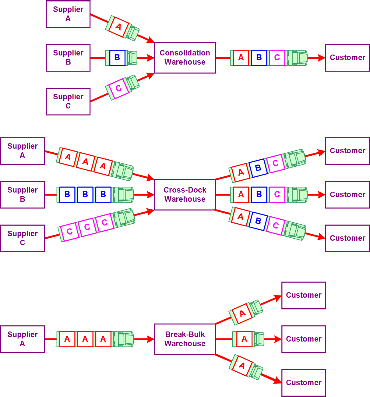
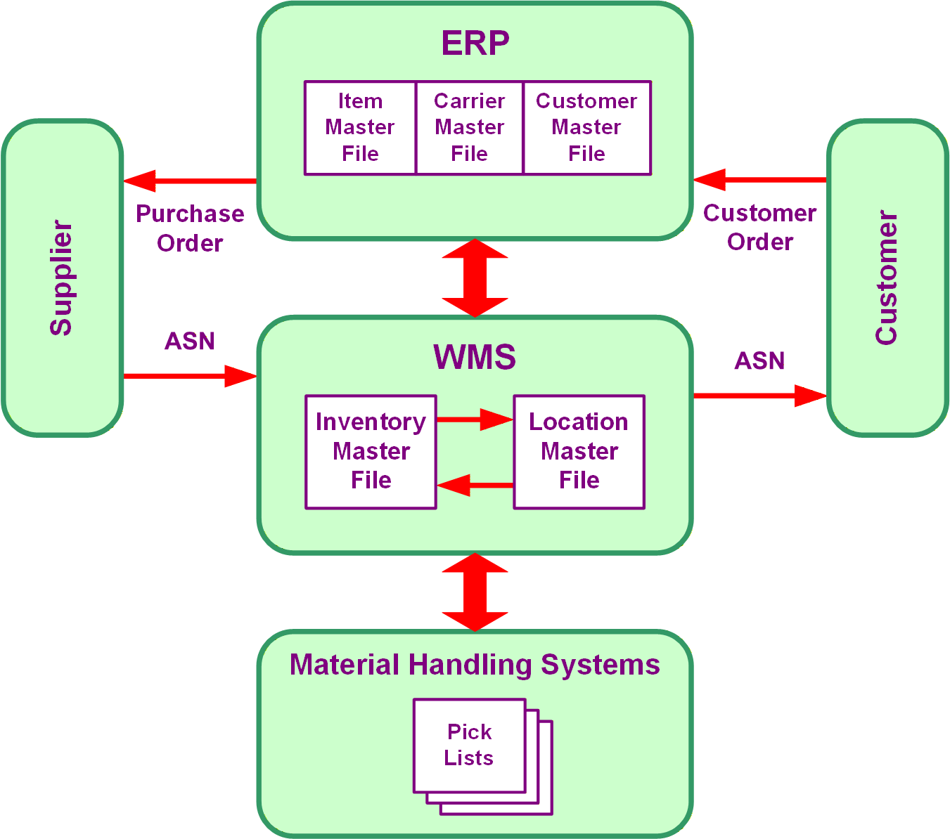
In transshipment, inventory is stored time: the gap between when freight arrives and when it is wanted. Cross-docking closes that gap by timing the arrivals, trading the cost of storage for the cost of coordination. That trade is made product by product.
No new Julia packages used.
New Logjam functions used
loc2lonlat: Geocode a single location string. Accepts addresses, city names, postal codes.
Companion script
3-tran-4.jl, runnable Julia extracted from the lecture’s code blocks.
1. Full-truckload location
A full-truckload (FTL) shipment is one whose size is the maximum payload, q = q_{\max}, while a truckload (TL) shipment can be any size up to it, q \le q_{\max}. As a result, FTL has two very useful features. The first is that most TL shipments should be close to FTL: it is not a good long-term strategy to ship half-empty trucks, and if necessary, a shipper can aggregate with other shipments to make it FTL. The second is that the monetary transport weights (w) and inventory cost (IC) are independent of the NF (new facility) location, so only the transport cost (TC) is needed for location analysis, unlike TL and less-than-truckload (LTL), which require total logistics cost (TLC).
Most of the time, a shipment should be a full truckload. Full truckloads are not a special case; they apply far more widely than they first appear, and they should be the main thing done. A truck shipped well short of its maximum payload wastes resources, and a company whose trucks are always half full will not stay in business long, unless what it ships, such as diamonds, has to be kept secure. When the optimal size of a general-freight shipment works out to half a truckload, the answer is not to send half-full trucks. It says that a private fleet is probably the wrong choice and that the shipper is a good candidate to hire a carrier, which can pick up the load and mix it with those of other customers nearby, so that the carrier’s own trucks run close to full. The allocated full truckload of Lecture 3.3, Sec. 2.3, gives the lower bound on what that should cost, the best case, and the independent, half-full shipment gives the upper bound; a contract negotiated with a carrier should land between the two, and where depends on the shipper’s bargaining power. A remote shipper with no other customers nearby has little leverage, since the carrier must send a truck for that load alone. Across most of the United States, though, the market of other shippers is thick enough that candidates for consolidation are almost always nearby.
A full truckload of a single, somewhat valuable product would carry so much inventory cost that it is not a good strategy; the way to fill a truck is to aggregate a shipment with others, either directly or by hiring a carrier, who combines many shippers’ loads, so that the shipper is in effect shipping aggregate shipments. With every shipment a full truckload, the monetary weights are constant, so the simple location techniques of the Location lectures apply as they stand. Once the optimal shipment size is calculated instead, it changes with the distance of the shipment, through the d in the optimal truckload size and in the LTL rate estimate, so every move of the candidate location means recalculating every shipment’s size. That is doable on a computer or even a spreadsheet, but not by hand. The full-truckload assumption is not just an artifact for solving location problems by hand, though. It has good engineering practice behind it, for the first reason: it is a happy coincidence that the assumption which allows a problem to be solved by hand is also what a real problem should face.
1.1 Weights from full truckloads
With every shipment a full truckload, the monetary weight of each facility shipping to or from a distribution center (DC) follows from its annual demand and its maximum payload alone, which is the full-truckload transport cost of Lecture 3.3, Sec. 2.1, written facility by facility:
=annual demand shipped to or from facility i (ton/yr)
r_{FTL,i}
=FTL rate for facility i’s shipments ($/ton-mi)
=r_i/q_{\max,i}
n_i
=shipment frequency to or from facility i (TL/yr)
=f_i/q_{\max,i}
r_i
=revenue per loaded truck-mile for facility i’s shipments ($/TL-mi)
q_{\max,i}
=maximum payload of facility i’s shipments (ton).
Because every w_i is fixed before the DC is placed, minimizing TC is the one-dimensional minisum problem of Model 8 in Lecture 2.1, solved by the weighted median.
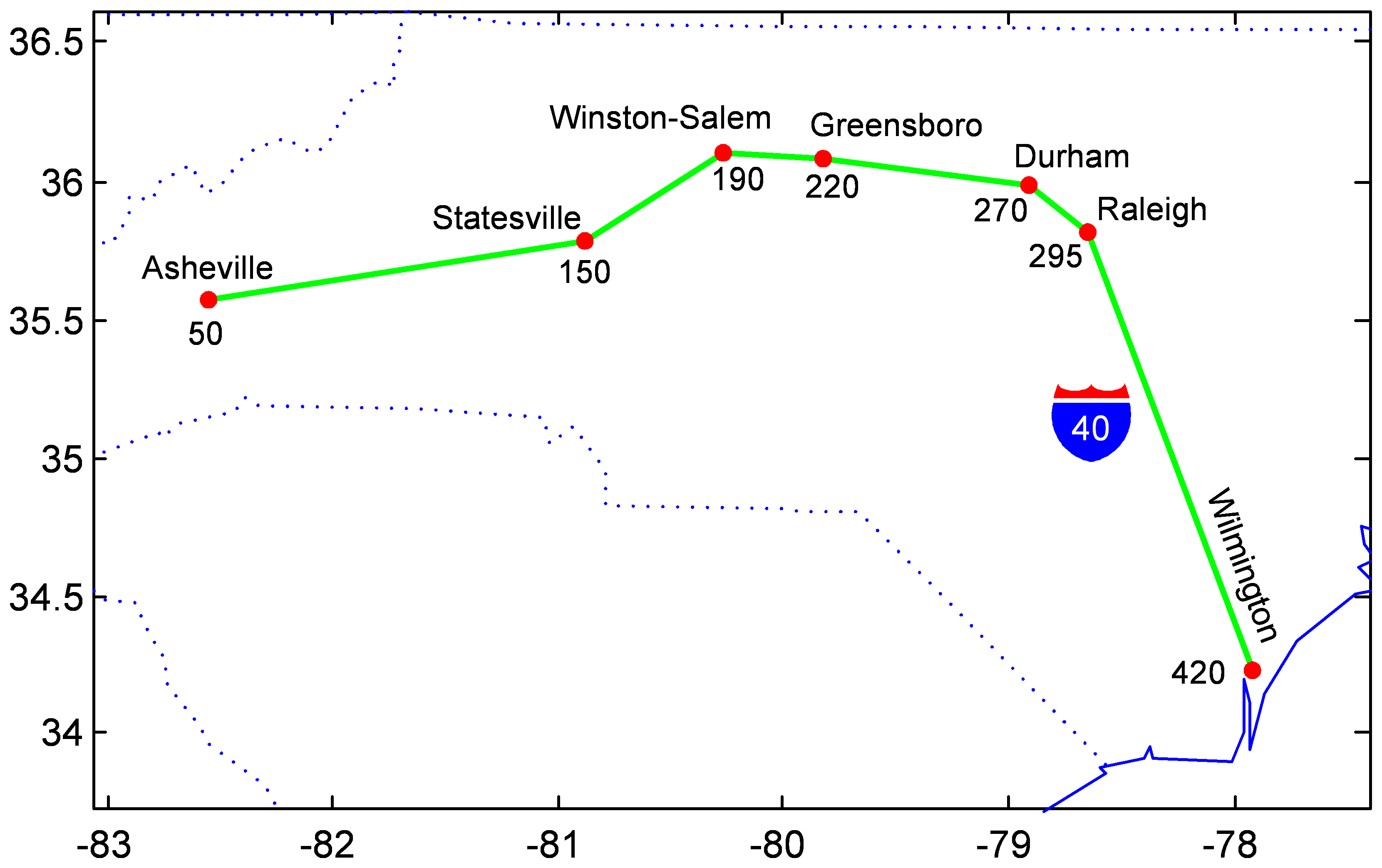
The worked example is the transshipment counterpart of Ex. 1 in Lecture 2.2, on the same stretch of I-40 (Fig. 1), with a DC in place of the plant.
Figure 1: The I-40 corridor with mile markers: Asheville (50), Statesville (150), Winston-Salem (190), Greensboro (220), Durham (270), Raleigh (295), and Wilmington (420).
Example 1: DC location along I-40
FTLs containing a mix of products A and B are shipped point-to-point (P2P) from a distribution center (DC) to customers in Winston-Salem, Durham, and Wilmington. Each customer receives 20, 30, and 50% of the total demand, respectively. The DC receives 100 ton/yr of A shipped FTL P2P from a supplier in Asheville and 380 ton/yr of B shipped FTL P2P from a supplier in Statesville. Each carton of A weighs 30 lb and occupies 10 ft3, and each carton of B weighs 120 lb and occupies 4 ft3. The revenue per loaded truck-mile is $2. Each truck’s cubic and weight capacity is 2,750 ft3 and 25 tons, respectively. The five facilities lie along I-40 at the mile markers shown in Fig. 1. Given these data, determine where the DC should be located in order to minimize transportation costs.
Products A and B do not change form in the DC; its only effect is on how they are transported. Unlike a manufacturing problem, where the demand for the finished product is given and the supply is worked back from it, here the supply of each product is given and only each customer’s share of the total demand is known. The customers could be other manufacturing facilities or actual locations rather than aggregate demand points, and for a retail product a good way to obtain the shares is from population: each customer’s ZIP code population as a percentage of the total market population. Every shipment here is a point-to-point (P2P) full truckload, which is not terribly realistic on I-40, since a full truck would drive straight past the stops where it could have picked up more. Multi-stop routing is the subject of the routing lectures, Lectures 5.1 to 5.3; for now the assumption stands. The key operation is at the DC. Each inbound truck carries a full truckload of a single product, A or B, and at the DC the two products are combined onto the same trucks to the customers. That is where the saving comes from: combining a very dense product with one that is not dense uses both the cube and the weight capacity of a truck better than either product could alone.
Example 1(a): From full truckloads to the monetary weights
Determine each facility’s monetary weight, inbound from the suppliers’ full truckloads and outbound from the customers’ shares of the aggregate product.
# Code block 1: the suppliers, the DC and the customers of Ex. 1nm = ["Asheville", "Statesville", "Winston-Salem", "Durham","Wilmington"]supc = colorant"#d21f26"# the suppliersdcc = colorant"#1e8a3c"# the DCcusc = colorant"#1f77c4"# the customersink = colorant"#252525"# A box with rounded corners, centered at (x, y), half-width a and# half-height bfunctionroundbox(x, y, a, b; c =0.08)arc(cx, cy, t0) = [Point2f(cx +c*cos(t), cy +c*sin(t)) for t inrange(t0, t0 +pi/2; length =8)] pts = Point2f[arc(x + a - c, y + b - c, 0);arc(x - a + c, y + b - c, pi/2);arc(x - a + c, y - b + c, pi);arc(x + a - c, y - b + c, 3pi/2)]return ptsendXY = [(0.0, 1.3), (0.0, 0.3), (3.0, 0.8), (6.0, 1.6), (6.0, 0.8), (6.0, 0.0)] # suppliers, DC, customerslab = [nm[1:2]; "DC"; nm[3:5]]col = [supc, supc, dcc, cusc, cusc, cusc]arcs = [(1, 3, "A, 100 ton/yr", :bottom), (2, 3, "B, 380 ton/yr", :top), (3, 4, "AB, 20%", :bottom), (3, 5, "AB, 30%", :bottom), (3, 6, "AB, 50%", :top)]a, b =0.68, 0.22# box half-width, half-height# Where a ray from a box's center along direction u leaves the boxedge(u) =min(a/max(abs(u[1]), 1e-9), b/max(abs(u[2]), 1e-9))fig =Figure(size = (687, 215))ax =Axis(fig[1, 1]; aspect =DataAspect())hidedecorations!(ax); hidespines!(ax)for (i, j, s, va) in arcs # each arc runs edge to edge p, q = XY[i], XY[j] u = (q .- p) ./hypot((q .- p)...) t, h = p .+edge(u) .* u, q .- (edge(u) +0.015) .* uarrows2d!(ax, [t[1]], [t[2]], [h[1] - t[1]], [h[2] - t[2]]; color = ink, shaftwidth =1.6, tipwidth =9, tiplength =9) m = (t .+ h) ./2text!(ax, m[1], m[2]; text = s, color = ink, fontsize =13, rotation =atan(u[2], u[1]), align = (:center, va), offset = (0, va ==:bottom ? 3:-3))endfor (i, (x, y)) inenumerate(XY)poly!(ax, roundbox(x, y, a, b); color =:white, strokecolor = col[i], strokewidth =1.8)text!(ax, x, y; text = lab[i], color = ink, fontsize =14, align = (:center, :center))endxlims!(ax, -0.8, 6.8); ylims!(ax, -0.35, 1.95)fig
Figure 2: The flows of Ex. 1. Products A and B arrive at the DC as single-product full truckloads from their suppliers, and each customer receives its share of the total demand as full truckloads carrying both.
# Code block 2: the products, the customers and their maximum payloadstr = (r =2, Kwt =25, Kcu =2750)uwt = [30, 120] # lb per carton, A and Bucu = [10, 4] # ft^3 per cartonshS =DataFrame(f = [100, 380], s = uwt./ucu) # the two supplierspct = [20, 30, 50]/100# each customer's share of demandsh =vcat(shS, DataFrame(f =sum(shS.f)*pct, s =sum(shS.f)./sum(shS.f./shS.s)))sh.qmax = [maxpayld(row, tr) for row ineachrow(sh)]prt(sh)
The statement leaves one assumption latent: each customer is taken to receive the two products in the same proportion. That is what allows a single aggregate product, its density and demand aggregated from the two suppliers’ shipments, to describe every outbound shipment in Code block 2.
# Code block 3: FTL truckloads and monetary weightsn = sh.f./sh.qmax # TL/yrw = n*tr.r # $/mi-yrprt(hcat(sh, DataFrame(n = n, w = w)))
f s qmax n w
──────────────────────────────────
1 100 3.00 4.12 24.24 48.48
2 380 30.00 25.00 15.20 30.40
3 96 10.43 14.35 6.69 13.38
4 144 10.43 14.35 10.04 20.07
5 240 10.43 14.35 16.73 33.45
Fig. 3 lays the same calculation out beside the facilities, as Lecture 2.2’s Ex. 1(a) does for its plant.
Show the code that draws this figure
# Code block 4: the monetary weights, computed beside their nodesfmt(x) = x ==round(x) ? string(Int(round(x))) :rstrip(rstrip(@sprintf("%.4f", x), '0'), '.')f2(x) =@sprintf("%.2f", x)frac(a, b) ="\\frac{$a}{$b}"fagg, sagg, qagg =sum(shS.f), sh.s[3], sh.qmax[3]# The canvas is laid out in pixels, so a font size is the size on the pagewpx, hpx, fsz, rn =687, 553, 16, 15xs, xdc, xc =290, 380, 470# node columns: in, DC, outxL, xR = xs - rn -12, xc + rn +12# where the two text columns enddy =36# one row of equationsydc =200ys = ydc .+ [112, -112] # suppliers 1 and 2yc = ydc .+ [124, 0, -124] # customers 3, 4 and 5yagg = [528, 483, 430] # the aggregate, over the DCfig =Figure(size = (wpx, hpx), figure_padding =0)ax =Axis(fig[1, 1]; aspect =DataAspect())hidedecorations!(ax); hidespines!(ax)# Each equation is set in math, as an L"..." string would beeq!(x, y, s, h) =text!(ax, x, y; text = Makie.LaTeXString("\$$s\$"), color = ink, fontsize = fsz, align = (h, :center))functionrows!(x, y, h, rs) # a block of rows centered on yfor (k, s) inenumerate(rs)eq!(x, y +dy*((length(rs) +1)/2- k), s, h)endreturnnothingendeq!(12, yagg[1], "r = \\\$$(tr.r)/\\mathrm{TL‑mi}", :left)for (y, e) inzip(yagg, [ # the aggregate, over the DC"f_{agg} = $(fmt(shS.f[1])) + $(fmt(shS.f[2])) = $(fmt(fagg))","s_{agg} = "*frac(fmt(fagg), frac(fmt(shS.f[1]), fmt(shS.s[1])) *" + "*frac(fmt(shS.f[2]), fmt(shS.s[2]))) *" = $(fmt(sagg))","q_{\\max} = \\min\\left\\{$(tr.Kwt), "*"$(frac("$(fmt(sagg))($(tr.Kcu))", 2000))\\right\\} = "*"$(fmt(qagg))"])eq!(xdc, y, e, :center)endfor k in1:2# the input side, left of 1 and 2 s, q =fmt(sh.s[k]), fmt(sh.qmax[k])rows!(xL, ys[k], :right, ["s_$k = $(frac(uwt[k], ucu[k])) = $s","q_{\\max} = \\min\\left\\{$(tr.Kwt), "*"$(frac("$s($(tr.Kcu))", 2000))\\right\\} = $q","f_$k = $(fmt(sh.f[k])), \\; n_$k = $(frac(fmt(sh.f[k]), q)) = "*"$(f2(n[k]))","w_$k = $(f2(n[k]))($(tr.r)) = $(f2(w[k]))"])endfor k in1:3# the output side, right of 3-5 i = k +2rows!(xR, yc[k], :left, ["f_$i = $(f2(pct[k]))f_{agg} = $(fmt(sh.f[i]))","n_$i = $(frac(fmt(sh.f[i]), fmt(qagg))) = $(f2(n[i]))","w_$i = $(f2(n[i]))($(tr.r)) = $(f2(w[i]))"])endfunctionflow!(p, q) # an arc touches both circles u = (q .- p) ./hypot((q .- p)...) t, h = p .+ rn .* u, q .- (rn +1) .* uarrows2d!(ax, [t[1]], [t[2]], [h[1] - t[1]], [h[2] - t[2]]; color = ink, shaftwidth =1.5, tipwidth =9, tiplength =9)returnnothingendfor k in1:2; flow!((xs, ys[k]), (xdc, ydc)); endfor k in1:3; flow!((xdc, ydc), (xc, yc[k])); endfunctionnode!(x, y, s, c)poly!(ax, Circle(Point2f(x, y), rn); color =:white, strokecolor = c, strokewidth =1.5)text!(ax, x, y; text = s, color = c, fontsize =14, align = (:center, :center))returnnothingendnode!(xs, ys[1], "1", supc); node!(xs, ys[2], "2", supc)node!(xdc, ydc, "DC", dcc)for k in1:3; node!(xc, yc[k], string(k +2), cusc); endxlims!(ax, 0, wpx); ylims!(ax, 0, hpx)fig
Figure 3: Computing the five monetary weights. The input side is on the left, beside suppliers 1 and 2, each shipping its own product as full truckloads; the output side is on the right, beside customers 3, 4 and 5, each receiving its share of the aggregate product formed at the DC, computed above it. Code block 3 carries out exactly these calculations.
Example 1(b): Locating the DC
Order the facilities along I-40 and apply the median procedure of Model 8 in Lecture 2.1.
With every weight known, the corridor is one-dimensional and the median procedure applies unchanged: sweep west to east, accumulate weight, and stop at the first facility where the running total reaches half the grand total.
The same answer comes by hand. Fig. 4 sets the monetary weights out in their order along I-40, and the running total, swept from either end, first passes half the total weight at Statesville.
Show the code that draws this figure
# Code block 6: the weighted median, swept from both endsrole = [:supplier, :supplier, :customer, :customer, :customer]functionweightline(w, nm, role) wc = colorant"#d21f26"# the weights chk = colorant"#1e8a3c"# the running checks opt = colorant"#b23a48"# the median m =length(w); W =sum(w); half = W/2 j =findfirst(>=(half), cumsum(w)) # the weighted median x =collect(1.0:m) # only the order matters issup = role .==:supplier fig =Figure(size = (687, 205)) ax =Axis(fig[1, 1])hidedecorations!(ax); hidespines!(ax)lines!(ax, [0.55, m +0.45], [0, 0]; color = ink, linewidth =2.5)scatter!(ax, x[issup], zeros(count(issup)); marker =:circle, markersize =14, color = supc)scatter!(ax, x[.!issup], zeros(count(.!issup)); marker =:rect, markersize =13, color = cusc)for i in1:mtext!(ax, x[i], 0.0; text = nm[i], color = ink, font =:bold, fontsize =14, align = (:center, :bottom), offset = (0, 34))text!(ax, x[i], 0.0; text =string(role[i]), color = issup[i] ? supc : cusc, fontsize =13, align = (:center, :bottom), offset = (0, 14))text!(ax, x[i], 0.0; text =f2(w[i]), color = wc, fontsize =14, align = (:center, :top), offset = (0, -12))end# The running total from each end, until it reaches half the total h =f2(half)check(c) ="$(f2(c))$(c < half ? "<":">")$h"for (row, idx) inenumerate((1:j, m:-1:j)) c =0.0for i in idx c += w[i]text!(ax, x[i], 0.0; text =check(c), color = chk, fontsize =13, align = (:center, :top), offset = (0, -36-20*(row -1)))endendtext!(ax, x[j], 0.0; text ="*", color = opt, fontsize =26, align = (:center, :top), offset = (0, -76))text!(ax, x[j], 0.0; text ="optimum (median)", color = opt, fontsize =13, align = (:center, :top), offset = (0, -100))text!(ax, 0.5, 0.0; text = L"w_i\;(\$/\mathrm{mi‑yr}):", color = wc, fontsize =13, align = (:right, :top), offset = (0, -12))text!(ax, 0.5, 0.0; text = L"\sum w_i \geq W/2:", color = chk, fontsize =13, align = (:right, :top), offset = (0, -46))text!(ax, m +0.45, 0.0; text ="W = $(f2(W)), W/2 = $h", color = ink, fontsize =13, align = (:right, :top), offset = (0, -100))xlims!(ax, -0.9, m +0.5); ylims!(ax, -1.08, 0.5)return figendweightline(w, nm, role)
Figure 4: The full-truckload monetary weights w_i ($/mi-yr) in their order along I-40, with the weighted-median search swept from both ends. Both running totals first reach half the total weight at Statesville (*), where the DC is located.
The DC is located at mile 150, Statesville, with a total transport cost of $16,825.21/yr.
Example 1(c): Weight-gaining or weight-losing
Classify the DC by comparing its inbound and outbound weights, physical and monetary.
Tons pass straight through a DC, and the weights do not. Totaling the inbound and outbound sides of the DC shows both, and the tons balancing is a Balance check of Lecture 1.2.
# Code block 7: tons, truckloads and weights in and out of the DCidxin, idxout =1:2, 3:5# suppliers in, customers out@showsum(sh.f[idxin]), sum(sh.f[idxout]) # ton/yr@showsum(n[idxin]), sum(n[idxout]) # TL/yr@showsum(w[idxin]), sum(w[idxout]) # $/mi-yr
Physically weight unchanging: 480 ton/yr in and 480 out. Monetarily weight losing: 78.88 $/mi-yr in against 66.91 out, 39.44 truckloads a year in against 33.45 out.
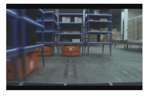
Measured by monetary weight the DC is weight losing, with more monetary weight coming in than going out, and in truckloads about 39 a year arrive from the suppliers while only about 33 leave for the customers. The six truckloads saved are the better utilization of each truck: product B weighs out and product A cubes out, and the aggregate of the two mixes them better. Physically nothing changes, since a DC is not a manufacturing plant with scrap or a ubiquitous input; the weight loss comes entirely from the difference between weighing out and cubing out, a trade-off that runs through every mode, air cargo, rail and ocean as much as trucking. Handling at the DC still costs something, and shipping directly to the customers is always the alternative. For a product that is fragile, or valuable enough to need high security, such as a costly pharmaceutical, the cost of unloading and handling at a DC can make point-to-point truckloads the better choice even when each truck is only a tenth full. That cost has been falling, though: led by Amazon and its Kiva robots, the cost of operating a warehouse has come down over the last ten to fifteen years, so handling is becoming less of a factor (Sec. 4.4).
NoteFull truckloads in practice
Is assuming full truckloads a gross error, made only because a one-dimensional location problem can then be solved by hand with a simple formula? For some products it does not hold at all. A company shipping blood plasma products, for example, might send a tractor-trailer across the country carrying a few hundred pounds, about 1% of its weight capacity, because the load is worth millions of dollars and getting it there is all that matters; the trailer is sealed and locked, since such trailers have been broken into for the value of what they carry. In general, though, shipments should be close to full truckloads. A business plan built on trucks that are 20% full and 80% wasted space, however well it minimized total logistics cost, would be rejected by any venture capitalist. Trucking is a thick market: a shipper whose trucks would run 80% empty is in effect running its own trucking company, and a small business should hire a carrier instead. The carrier has many other customers and runs close to full all the time, with the shipper’s goods perhaps one of 20 customers’ loads on a truck, so the goods effectively ship as a full truckload even though the shipper is not the one making the decision to ship that way. Outside a really isolated area, a plan that ships a truck 80% air is a red flag that something is wrong with the analysis.
FTL, since its size is fixed at the maximum payload, results in only constant weights for location, so there is a need to only minimize TC, since IC is constant in TLC:
=inventory fraction of Lecture 3.3, Sec. 3 (dimensionless)
v
=unit value ($/ton)
h
=inventory carrying rate (1/yr)
TLC_{FTL}(\mathbf{x})
=total logistics cost with every shipment a full truckload ($/yr)
TC_{FTL}(\mathbf{x})
=transport cost with every shipment a full truckload ($/yr).
1.2 Minimum outbound frequency
As an extension, Ex. 1 can include a monthly outbound frequency constraint: outbound shipments must occur at least once each month. The constraint provides an implicit means of including inventory costs in the location decision. With at most a month between shipments, each customer receives at least 12 truckloads a year:
Fig. 5 repeats the weighted-median search with the new weights.
Show the code that draws this figure
weightline(w′, nm, role) # Code block 9: the search with the floor
Figure 5: The monetary weights w'_i ($/mi-yr) with at least one outbound shipment a month. The running total first reaches half the total weight at Winston-Salem (*), where the DC is now located.
The DC moves to mile 190, Winston-Salem. The floor adds 7.27 truckloads a year, and the total transport cost at the new location is $17,618.42/yr, against $16,825.21/yr without it.
In addition to the change of location, the total transport costs increase due to the increase in the number of shipments. The increase in cost could also be calculated by hand, but this would require having to determine distances, which is tedious; it is the last line of Code block 8. The DC moving east, toward the customers whose weights the floor raised, is the direction the change should push it, which is the Nudge check of Lecture 1.2.
The constraint changes only some of the numbers. The customer with the highest demand already receives more than 12 truckloads a year and passes through unchanged; the other two receive fewer than 12, so their shipments rise to 12 a year and their monetary weights are recalculated. The total weight becomes 160, and the DC moves from Statesville to Winston-Salem. Measured by monetary weight, the DC is now weight gaining. The demand has not changed, but deliveries to the smallest customer nearly double, so a truck to that customer runs about half empty and the outbound side uses its trucks less efficiently. That is very typical of a DC, with truckloads coming in and smaller, more expensive delivery vans going out. A DC with rail coming in and trucks going out is always weight gaining, since rail is so much cheaper on a monetary-weight basis; a DC is weight losing only when the same mode is used in and out and the frequency does not change, so that aggregation is the only effect. Whether more frequent deliveries are worth it cannot be determined from this problem, because it does not compute the total logistics cost. Ex. 2 in Lecture 3.3 did, and gave a dollar figure for the impact of a shorter shipment interval, the number a negotiation or a business analysis would start from.
Full truckloads to every customer may not be the whole situation, since a customer may want a monthly outbound frequency written into its contract. At present the first customer receives a shipment only about every two months, the second almost every month, and the third more than once a month, so the constraint does not affect the customers equally: it nearly doubles the shipments to the first, the customer with the lowest demand, and leaves the third, with half the demand, as it was. The example is set up with both suppliers in the west and the three customers in the east precisely so that the constraint makes a visible change; with suppliers and customers mixed along the route, it would probably not move the DC. Weight gaining is the more common case for a DC, since deliveries to customers typically face more stringent interval constraints and go in smaller trucks, more frequently. Physically, a DC usually changes little, but not always. Product can be lost, such as units that arrive damaged and cannot be repaired, and product can be added: it can be cheaper to do the last steps at the DC, such as filling something with a fluid that would be expensive to transport, or a limited final assembly. Beach balls and basketballs, for example, do not come from China inflated; every Walmart DC has a station that inflates them before they go on to the stores. Kitting at the DC, a limited assembly, sits between a product shipped assembled and flat-packed furniture assembled at home, and it is done for the transport efficiency. Once looked for, the phenomenon appears almost everywhere: the trade-off between cube and weight is the story behind many of the ways things are done in a supply chain.
Ex. 1 continues in Sec. 2.3, where the shipments to and from the DC are no longer full truckloads.
2. Transshipment
2.1 Direct and transshipment
Direct shipment means P2P shipments from suppliers to customers, as on the left of Fig. 6. Transshipment is the use of a DC to consolidate outbound shipments, as on the right, and it runs in one of two ways. Uncoordinated transshipment determines separately each optimal inbound and outbound shipment, and so it must hold inventory at the DC. A (perfect) cross-dock uses a single shipment interval for all inbound and outbound shipments, so there is no inventory at the DC; a non-perfect cross-dock would only cross-dock a selected subset of shipments.
Show the code that draws this figure
# Code block 10: direct and transshipment networks# Each arc: from, to, its products, where along it the label sits, and# whether the label sits above or below it.functionnetwork!(ax, XY, nm, arcs) acol, bcol = colorant"#d21f26", colorant"#1e8a3c"# product A, B rn =0.17# node radius, in data unitsfor (i, j, lab, s, va) in arcs p, q = XY[i], XY[j] u = (q .- p) ./hypot((q .- p)...)# Each arc starts on one circle and ends on the other a, b = p .+ rn .* u, q .- (rn +0.015) .* uarrows2d!(ax, [a[1]], [a[2]], [b[1] - a[1]], [b[2] - a[2]]; color = ink, shaftwidth =1.5, tipwidth =9, tiplength =9) m = p .+ s .* (q .- p) txt = [rich(string(c); color = c =='A' ? acol : bcol) for c in lab]text!(ax, m[1], m[2]; text =rich(txt...), fontsize =15, font =:bold, align = (:center, va), offset = (0, va ==:bottom ? 4:-4))end# Circles drawn in data units, so the radius the arcs stop at is the# radius drawn; a marker sized in pixels never matches itfor (x, y) in XYpoly!(ax, Circle(Point2f(x, y), rn); color =:white, strokecolor = colorant"#1f77c4", strokewidth =1.5)endtext!(ax, first.(XY), last.(XY); text = nm, fontsize =14, color = ink, align = (:center, :center))return axendfig =Figure(size = (687, 210))for (c, title) inenumerate(["Direct", "Transshipment"]) ax =Axis(fig[1, c]; title = title, titlefont =:regular, titlesize =15, aspect =DataAspect())hidedecorations!(ax); hidespines!(ax)if c ==1network!(ax, [(0.0, 1.0), (0.0, 0.0), (2.4, 1.0), (2.4, 0.0)], ["1", "2", "3", "4"], [(1, 3, "A", 0.5, :bottom), (1, 4, "A", 0.3, :bottom), (2, 3, "B", 0.3, :bottom), (2, 4, "B", 0.5, :top)])elsenetwork!(ax, [(0.0, 1.0), (0.0, 0.0), (1.2, 0.5), (2.4, 1.0), (2.4, 0.0)], ["1", "2", "DC", "3", "4"], [(1, 3, "AA", 0.5, :bottom), (2, 3, "BB", 0.5, :top), (3, 4, "AB", 0.5, :bottom), (3, 5, "AB", 0.5, :top)])endtext!(ax, -0.35, 0.5; text ="Suppliers", rotation =pi/2, fontsize =13, color = ink, align = (:center, :center))text!(ax, 2.75, 0.5; text ="Customers", rotation =pi/2, fontsize =13, color = ink, align = (:center, :center))xlims!(ax, -0.5, 2.9); ylims!(ax, -0.25, 1.3)endfig
Figure 6: Two suppliers and two customers. Shipped direct, each supplier sends its single product to each customer; with transshipment, each supplier ships its product to a DC, where products A and B are combined into each outbound load.
In this distribution problem each customer wants both products A and B, which are not combined into a different product as they would be in manufacturing. Shipped direct, every supplier ships to every customer; with transshipment, the DC lets each outbound shipment carry a mix of the two products. Transshipment can be run at two extremes. At one, termed uncoordinated, the shipment from each supplier is determined to be optimal for that supplier and the shipment to each customer optimal for that customer, with no coordination between when products arrive at the DC and when they are demanded from it. At the other, perfect cross-docking, all inbound shipments have the same shipment interval: everything arrives at the DC, say, once a week, is offloaded onto the floor rather than put into storage racks, and is immediately switched around and shipped out to the customers, much as at an LTL terminal. The advantage is that no inventory is held at all. The difficulty is that every shipment must arrive on time, which would have taken good luck thirty years ago; tracking has made it better, but things still happen. So most cross-docking in practice is non-perfect: the subset of products that can benefit most is identified and cross-docked, and the rest is probably better left uncoordinated. Neither extreme is likely to be what a DC actually does, but an example of each shows how the two compare.
2.2 Inventory at a DC
Uncoordinated transshipment holds stock at the DC, and the average in-transit inventory level at the DC is counted in the inventory fraction \alpha of Lecture 3.3, Sec. 3, by splitting it between the inbound and the outbound shipments:
=inventory fraction held at the supplier (dimensionless)
\alpha_C
=inventory fraction held at the customer (dimensionless).
\alpha is the inventory fraction of Lecture 3.3, Sec. 3. \alpha_S is 0 for batch production and \tfrac{1}{2} for constant production; \alpha_C is 0 when a shipment is used on arrival and \tfrac{1}{2} for constant consumption.
Fig. 7 shows why one half is the right fraction for the DC.
Show the code that draws this figure
# Code block 11: the inventory profile at the DCT =27# periods showntS = ([2, 9, 16, 23], [1, 6, 11, 16, 21, 26]) # arrivals of A, of BqS = (3, 2) # q*_A and q*_BtC = ([3, 10, 17, 24], [4, 8, 12, 16, 20, 24]) # to customers 3, 4# The level after each event, and its average over the T periodsfunctionprofile(ts, q, tc, T) ev =sort(unique([0; ts; reduce(vcat, tc); T])) lev = [q*count(<=(t), ts) -sum(count(<=(t), c) for c in tc) for t in ev] avg =sum(lev[1:end-1] .*diff(ev))/Treturn ev, lev, avgendprof = [profile(tS[k], qS[k], tC, T) for k in1:2]fig =Figure(size = (687, 360))blue = colorant"#1f77c4"; grn = colorant"#1e8a3c"; red = colorant"#d21f26"for k in1:2 ev, lev, avg = prof[k] ax =Axis(fig[k, 1]; ylabel ="Supplier $k", yticks =0:qS[k]+1, ylabelsize =13, yticklabelsize =12, ylabelrotation =0, xgridvisible =false)hidexdecorations!(ax); hidespines!(ax, :t, :r)stairs!(ax, ev, lev; step =:post, color = blue, linewidth =2)hlines!(ax, [qS[k]/2]; color = red, linestyle =:dot, linewidth =1.5)scatter!(ax, tS[k], zeros(length(tS[k])); marker =:xcross, color = grn, markersize =13)xlims!(ax, 0, T); ylims!(ax, -0.3, maximum(lev) +0.4) a =@sprintf("%.2f", avg) p = k ==1 ? L"%$a\approx q_A^*/2": L"%$a\approx q_B^*/2"Label(fig[k, 2], p; fontsize =15, color = ink, halign =:left)endfor (c, ts) inenumerate(tC) ax =Axis(fig[2+ c, 1]; ylabel ="Customer $(c +2)", ylabelsize =13, ylabelrotation =0, xgridvisible =false)hideydecorations!(ax, label =false); hidespines!(ax, :t, :r, :l)if c ==1hidexdecorations!(ax); hidespines!(ax, :b)else ax.xlabel ="time"; ax.xlabelsize =13; ax.xticklabelsize =12endhlines!(ax, [0]; color = ink, linewidth =1)scatter!(ax, ts, zeros(length(ts)); marker =:xcross, color = red, markersize =13)xlims!(ax, 0, T); ylims!(ax, -0.6, 0.6)endrowsize!(fig.layout, 1, Relative(0.34))rowsize!(fig.layout, 2, Relative(0.26))fig
Figure 7: Inventory at a DC under uncoordinated transshipment. Supplier 1 ships q_A^* = 3 units of A and supplier 2 ships q_B^* = 2 units of B (green ×) on their own schedules, and every shipment to customer 3 or 4 takes one unit of each (red ×). The average inventory of each product at the DC is close to half its inbound shipment size (dotted).
The periodic shipments of Lecture 3.3 had one origin and one destination; at a DC, inbound and outbound shipments are coupled. The way to handle that is to separate the inventory fraction into its inbound and outbound parts. On the inbound side, \alpha_S is the inventory at the supplier: zero for batch production and one half for constant production. The average inventory at the DC turns out to be one half of each inbound shipment, and where that half is placed is arbitrary: on the inbound side, as in Eq. 4, with nothing added on the outbound side, or the other way round, or split, so long as the total nets out the same. On the outbound side, \alpha_C depends on how the customer consumes the product, immediately or at a constant rate. The half is placed on the inbound side because production is typically in batches and consumption constant, so that both sides come to one half and \alpha is one half on every shipment, which is convenient once the shipments are rows of a DataFrame. Nor is the half an arbitrary choice. It was first checked by simulation, and Fig. 7 reduces that check to a small deterministic picture: with optimal shipment sizes of 3 units of A and 2 of B, and every outbound shipment taking one unit of each, the average inventory of each product at the DC is close to half its inbound shipment size, 1.5 for A and 1 for B. That is the justification for one half: it matches what actual inventory profiles show, and it works in practice.
2.3 Single-DC transshipment
With a DC between the suppliers and the customers, each product is either cross-docked or stocked at the DC, and Model 1 states the problem of determining which.
A cross-docking set is a group of products whose suppliers all ship on one interval, the set’s own, so that its products arrive at the DC together and leave it the same day. A product in no set is stocked: held at the DC, and shipped in on its own interval. A delivery is everything a customer receives from the DC on one day. Each set makes a delivery to each customer on its interval, and a stocked product goes out either in one set’s deliveries or in a delivery that carries only stocked products. A shipment is uncoordinated when its size is its own optimal size, as in Lecture 3.3, and coordinated when its size is its annual flow times its set’s interval. Every shipment is therefore one of the four kinds in Table 1.
Table 1: The four kinds of shipment through the DC, in or out and uncoordinated or coordinated, each with its inventory fraction.
delivery that carries only stocked products (\alpha_C)
set’s delivery, with any stocked products it carries (\alpha_C)
The two columns differ in what one truck means. An uncoordinated shipment never needs more than one: two truckloads sent together cost the same transport as two sent on different days, since the TL charge of Eq. 9 in Lecture 3.2 counts every truck, but they double the inventory, which is why Eq. 2 in Lecture 3.3 holds a periodic shipment to one truck. A coordinated shipment can be larger. One in from a supplier is still held to one truck, which limits how long its set’s interval can be. A set’s delivery that is larger than one truck goes as two or more shipments on the same day, since its products arrived together and leave together.
minimize: total logistics cost of transporting the products from their suppliers through the DC to the customers, transport plus cycle inventory
solve for:
(a) sets of products cross-docked together, no product in two sets, and products in no set stocked at the DC (with no sets, every product is stocked);
(b) shipment interval of each set, and shipment size of each uncoordinated shipment;
(c) for each stocked product, the set, if any, whose deliveries to the customers also carry it.
subject to:
(a) payload: no shipment is larger than one truck’s maximum payload;
(b) interval: each set’s interval is at least one day.
assumptions:
(a) DC location is given;
(b) each supplier’s and each customer’s inventory fraction, \alpha_S and \alpha_C, is given;
(c) every shipment is an independent shipment;
(d) stocked products are held at the DC, and the products of each set arrive at it together and leave it the same day.
Model 1: Single-DC transshipment
The decision is a split of the products: a set S stocked at the DC, and a collection \mathcal{G} of sets, the products of each set cross-docked together on its own interval, and the stocked products, if any, that each set’s deliveries also carry. Its shipments are the four kinds of Table 1, and the problem is to find the split of least total cost:
=size of shipment or delivery i (decision variable, ton)
I
=shipments in from the suppliers, and deliveries out
TLC_i(q)
=total logistics cost of shipment or delivery i at size q ($/yr)
I_S
=shipments in from the suppliers
q_{\max,i}
=maximum payload of shipment i (ton)
t_G
=shipment interval of set G (decision variable, yr)
\mathcal{G}
=cross-docking sets, no product in two (decision variable)
t_{\min}
=shortest interval, one day (yr)
=1/365.25
f_i
=annual flow of shipment or delivery i (ton/yr)
I_G
=shipments in of the products in G, and deliveries out of G \cup S_G
S_G
=stocked products in G’s deliveries (decision variable).
A model states its constraints in words, under subject to, and its formulation writes each one as a row with the same letter. Model 1’s two constraints, (a) payload and (b) interval, are about shipments: what a truck carries, and how often a set ships. Both are rows here, (a) for the shipments in from the suppliers and (b) for each set. A delivery needs no row (a), since one larger than a truck goes as two or more shipments.
The row with no letter is not among Model 1’s constraints: it puts each set’s coordinated shipments, I_G, on the set’s interval. The sets \mathcal{G} of solve-for (a) and the stocked products S_G of solve-for (c) need no rows of their own; they determine which deliveries make up I and I_G, and what each carries.
With \mathcal{G} empty, every product is stocked, which is Model 2; with S empty and \mathcal{G} a single set, every product is cross-docked together, which is Model 3. The formulation says how any split is evaluated and nothing about how to search for a good one; Model 1 has no implementation here, on purpose.
In practice it is difficult to put every shipment on a single interval: the DC would sit empty most of the day, and then everything would arrive, be cross-docked and leave within a two-hour window. What happens at most DCs is a mix of stocked and cross-docked products, and the cross-docked products are usually not a single set. Coordination makes sense for certain high-value products, while low-value, more general products are probably best left uncoordinated. Seasonal goods are a classic case. A large retailer’s DC does not receive Halloween products from January on and fill a warehouse with them; they arrive over the month or two before the holiday, and a container or truckload of them, once unloaded, is not put into storage, because the stores need it quickly. It is cross-docked at once, one truckload holding enough to supply perhaps 20 to 25 stores, as whole pallets that go straight onto the store floor and are opened there. The trend is toward ever more cross-docking, since cross-docking needs good coordination and companies have become better at tracking their shipments.
This lecture solves Model 1 only at its two extremes, every product stocked and every product cross-docked in one set. The first is uncoordinated transshipment:
minimize: total logistics cost of transporting the products from their suppliers through the DC to the customers, transport plus cycle inventory
solve for:
(a) sets of products cross-docked together, no product in two sets, and products in no set stocked at the DC (with no sets, every product is stocked);
(b) shipment interval of each set, and shipment size of each uncoordinated shipment;
(c) for each stocked product, the set, if any, whose deliveries to the customers also carry it.
subject to:
(a) payload: no shipment is larger than one truck’s maximum payload;
(b) interval: each set’s interval is at least one day; (c) stocked: no sets, so every product is stocked at the DC.
assumptions:
(a) DC location is given;
(b) each supplier’s and each customer’s inventory fraction, \alpha_S and \alpha_C, is given;
(c) every shipment is an independent shipment;
(d) stocked products are held at the DC, and the products of each set arrive at it together and leave it the same day.
With every product stocked, every shipment is uncoordinated, with its own optimal shipment size, found as Lecture 3.3 found it for a single P2P shipment, with the DC’s inventory counted on the inbound side by Eq. 4:
=shipments in from the suppliers and out to the customers
TLC_i(q)
=total logistics cost of shipment i at size q ($/yr)
q_{\max,i}
=maximum payload of shipment i (ton).
Model 2 states three constraints in words, and its formulation writes each one it needs as a row with the same letter. It needs only one. Row (a) is the payload constraint: each shipment fits in one truck. Constraint (b) limits the interval of a cross-docked set, and with every product stocked, which is constraint (c), there is no such set, so neither needs a row. Stocking does show up in the costs, as the DC’s inventory in the inbound fraction of Eq. 4.
No term of the objective and no row involves two shipments, so the program separates into one P2P problem per shipment, each the minimization of Eq. 17 in Lecture 3.3 that Lecture 3.3 solved for a single shipment. Its solution is the sizes q_i^{\star}, and its minimum, TLC_{UC} = \sum_{i \in I} TLC_i(q_i^{\star}), is the cost of Eq. 5 with no cross-docking sets, every product stocked.
No Logjam function computes either extreme, so each implementation is written out here. The one new piece is the transport charge of a supplier or customer located at the DC itself, which is zero, since the product moves to the DC without a truck.
Model 2 implementation: Uncoordinated transshipment
# Model: uncoordinated transshipment# Independent transport charge: TL, or the cheaper of TL and LTL when an# LTL PPI is given; zero when the distance is zero (no truck is needed)functionc0(q, sh, tr, ppi =nothing)isapprox(sh.d, 0, atol =1e-4) &&return0.0 c =charge_tl(q, sh, tr)return ppi ===nothing ? c :min(c, charge_ltl(q, sh; ppi = ppi))end# The minimum-TLC size of every shipment on its ownfunctiontlc_uc(sh, tr, ppi =nothing) q = [isapprox(r.d, 0, atol =1e-4) ? 0.0:minTLC(r, tr, ppi).qᵒ for r ineachrow(sh)] TLC =sum(totlogcost(q[i], c0(q[i], r, tr, ppi), r)for (i, r) inenumerate(eachrow(sh)))return (TLC = TLC, q = q)end
tlc_uc (generic function with 2 methods)
The other extreme is perfect cross-docking, every product cross-docked in one set:
minimize: total logistics cost of transporting the products from their suppliers through the DC to the customers, transport plus cycle inventory
solve for:
(a) sets of products cross-docked together, no product in two sets, and products in no set stocked at the DC (with no sets, every product is stocked);
(b) shipment interval of each set, and shipment size of each uncoordinated shipment;
(c) for each stocked product, the set, if any, whose deliveries to the customers also carry it.
subject to:
(a) payload: no shipment is larger than one truck’s maximum payload;
(b) interval: each set’s interval is at least one day; (c) single set: every product is cross-docked, all in one set.
assumptions:
(a) DC location is given;
(b) each supplier’s and each customer’s inventory fraction, \alpha_S and \alpha_C, is given;
(c) every shipment is an independent shipment;
(d) stocked products are held at the DC, and the products of each set arrive at it together and leave it the same day.
Under perfect cross-docking every shipment is coordinated, so the shipment sizes cannot be found one at a time: every shipment shares one interval t. The key is that a shipment’s size is then its annual flow times that interval, q_i = f_i t, so one interval fixes every size. The formulation keeps the objective of Eq. 6 and adds that relation as row (c):
=size of shipment or delivery i (decision variable, ton)
I
=shipments in from the suppliers, and deliveries out
TLC_i(q)
=total logistics cost of shipment or delivery i at size q ($/yr)
I_S
=shipments in from the suppliers
q_{\max,i}
=maximum payload of shipment i (ton)
t
=common shipment interval (decision variable, yr)
t_{\min}
=shortest interval, one day (yr)
=1/365.25
f_i
=annual flow of shipment or delivery i (ton/yr).
Model 3 states the same three constraints, and here all three are rows. Row (a), payload, is the row of Eq. 5, for the shipments in from the suppliers. Row (b), interval, keeps the common interval to at least one day. Row (c), single set, puts every shipment and delivery on that one interval, so each one’s size is its annual flow times the interval. With nothing held at the DC, each shipment’s inventory fraction is \alpha_S inbound and \alpha_C outbound. Rows (a) and (c) together also cap the interval: a shipment in from a supplier fills its truck at t = q_{\max,i}/f_i, so t can be no longer than the shortest of these, which is the upper end of the implementation’s search:
Set beside Eq. 6, the objective is the same, row (a) is written only for the shipments in from the suppliers, and Model 3 adds rows (b) and (c). Row (c) ties every size to one variable, so the program no longer separates, and the search is over t alone. Its solution is the interval t^{\star}, the sizes follow as q_i^{\star} = f_i\, t^{\star}, and its minimum, TLC_{XD} = \sum_{i \in I} TLC_i(q_i^{\star}), is the cost of Eq. 5 with every product in a single cross-docking set.
The implementation prices every shipment with the charge c0 of Model 2.
Model 3 implementation: Perfect cross-docking
# Model: perfect cross-docking# One interval t for every shipment, q = f t; c0 from uncoordinated# transshipmentfunctiontlc_xd(sh, tr, tmin, tmax, ppi =nothing)TLC(t) =sum(r ->totlogcost(r.f*t, c0(r.f*t, r, tr, ppi), r),eachrow(sh)) t =optimize(TLC, tmin, tmax).minimizer # (b) below; (a), (c) abovereturn (TLC =TLC(t), t = t, q = sh.f*t)end
tlc_xd (generic function with 2 methods)
Example 1(e): Uncoordinated inventory at Statesville
Continuing with Ex. 1, all transport is TL (no LTL). Each carton of A is valued at $300, and each carton of B is valued at $450; the suppliers have batch production, and the customers constant consumption. Transshipments at the DC use either uncoordinated inventory (UC) or perfect cross-docking (XD). Determine the total logistics cost of uncoordinated inventory with the DC at Statesville, where Ex. 1(b) located it.
Total logistics cost needs the value of each product per ton, which follows from the value and weight of its carton, for product A:
=unit value: the value of one carton of A ($/carton)
\mathit{wt}_A
=unit weight: the weight of one carton of A (lb/carton).
With batch production at the suppliers and constant consumption at the customers, Eq. 4 gives one half on every shipment.
# Code block 12: values, inventory fractions and the carrier's PPItr = (r =2, Kwt =25, Kcu =2750, ppi =102.7) # MC = $45, Lecture 3.2uval = [300, 450] # $ per carton, A and BshS.v = uval./(uwt/2000) # $/tonαS =0# batch productionshS.a .= αS +0.5# uncoordinated DCshC =DataFrame(f =sum(shS.f)*pct, s =sum(shS.f)./sum(shS.f./shS.s), v =sum(shS.f.*shS.v)/sum(shS.f))shC.a .=0.5# constant consumptionsh =vcat(shS, shC)sh.h .=0.3# 1/yr, a default carrying rateprt(sh)
f s v a h
────────────────────────────────────────
1 100 3.00 20,000.00 0.5000 0.3000
2 380 30.00 7,500.00 0.5000 0.3000
3 96 10.43 10,104.17 0.5000 0.3000
4 144 10.43 10,104.17 0.5000 0.3000
5 240 10.43 10,104.17 0.5000 0.3000
The distance from a DC at mile x to each facility is computed from the I-40 mile markers of Code block 5.
# Code block 13: shipments with their distances from a DC at xshd(x) =hcat(sh, DataFrame(d = [d1.(x, P[idxin]); d1.(x, P[idxout])]))prt(shd(0))
f s v a h d
─────────────────────────────────────────────
1 100 3.00 20,000.00 0.5000 0.3000 50
2 380 30.00 7,500.00 0.5000 0.3000 150
3 96 10.43 10,104.17 0.5000 0.3000 190
4 144 10.43 10,104.17 0.5000 0.3000 270
5 240 10.43 10,104.17 0.5000 0.3000 420
The charge c0 in the implementation of Model 2 is 0 if the distance of a shipment is 0 to allow the DC to be located at an existing facility (EF) and thus incur no transport charges. This assumes all EFs are actual facilities and not aggregate demand points.
One change to the TL transport charge is important. The demand here is not aggregate demand spread over a region; every facility is an actual physical location. A DC located at the Statesville supplier should then not have to incur the TL minimum charge, which is independent of distance. A minimum charge makes sense for a shipment of one mile, but not when the distance is essentially zero. So the charge is set to zero when the distance is approximately zero: a DC in the same building as the supplier needs no truck at all, and the product is simply taken from one place to the other.
# Code block 14: uncoordinated TLC with the DC at StatesvilleTLCh(x) =tlc_uc(shd(x), tr).TLCxᵒ =150# Statesville@show TLC_UC =TLCh(xᵒ) # $/yrshUC =shd(xᵒ)shUC.qmax = [maxpayld(r, tr) for r ineachrow(shUC)]shUC.qᵒ =tlc_uc(shUC, tr).qshUC.TLCᵒ = [totlogcost(r.qᵒ, c0(r.qᵒ, r, tr), r) for r ineachrow(shUC)]prt(shUC)
Uncoordinated inventory with the DC at Statesville costs $64,820.57/yr in total logistics cost, nothing of it on the shipment from the Statesville supplier.
Example 1(f): Perfect cross-docking at Statesville
Determine the total logistics cost of perfect cross-docking with the DC at Statesville, and the common shipment interval that minimizes it.
To simplify, the example uses the optimal UC location (Statesville, as Ex. 3(a) shows), which may not be optimal for XD. As a result, it can use the final shUC from UC since it has a column d with the distance from the optimal UC location to each EF. shUC is copied to a new DataFrame shXD so that the a column can reflect cross-docking (it cannot just add another column to sh because totlogcost is looking for the a column). The upper end of the search is t_{\max} of Eq. 8, taken over the inbound shipments, idxin.
# Code block 15: perfect cross-docking with the DC at StatesvilleshXD = shUC[:, Not([:qᵒ, :TLCᵒ])]shXD[idxin, :a] .= αS # outbound α is unchangedtmax =minimum(shXD.qmax[idxin]./shXD.f[idxin]) # yr, inbound onlyxd =tlc_xd(shXD, tr, 1/365.25, tmax)@show xd.t, 365.25xd.t # yr, daysshXD.qXD = xd.qshXD.TLC_XD = [totlogcost(r.qXD, c0(r.qXD, r, tr), r) for r ineachrow(shXD)]@show xd.TLC # $/yr
Perfect cross-docking at Statesville ships every 13.94 days and costs $55,539.18/yr, against $64,820.57/yr for uncoordinated inventory.
One problem remains: the solution is not realistic because both UC and XD shipments are using only a small portion of the maximum TL payload. There are two fixes. One is to include LTL as a transport option, although its 35 mi distance limit is a problem on these short distances. The other is to consider the current XD solution as an upper bound (UB) on TLC and use the allocated FTL charge as a lower bound (LB):
\begin{aligned}
r_{FTL} &= \frac{r_{TL}}{q_{\max}} \\
TLC_{\text{AllocFTL}} ( q_{TL}^{\star} ) &= \frac{f}{q_{TL}^{\star}} ( q_{TL}^{\star} r_{FTL} d ) + \alpha v h\, q_{TL}^{\star} \\
&= f \frac{r_{TL}}{q_{\max}} d + \alpha v h\, q_{TL}^{\star}
\end{aligned}
\tag{10}
where
r_{FTL}
=allocated full-truckload rate ($/ton-mi)
r_{TL}
=TL revenue per loaded truck-mile ($/mi)
q_{TL}^{\star}
=shipment size at which the bound is evaluated (ton)
TLC_{\text{AllocFTL}}
=allocated full-truckload logistics cost ($/yr).
Here q_{TL}^{\star} is each shipment’s cross-docked size, and each shipment pays only its share of a full truckload. This is the allocated full-truckload cost of Eq. 20 in Lecture 3.3, the bottom of the range of possible transport charges in Fig. 1 in Lecture 3.3.
Example 1(g): Bounds on the total logistics cost
Determine the allocated full-truckload total logistics cost at the cross-docked shipment sizes, as a lower bound on what the DC at Statesville should cost.
# Code block 16: allocated full-truckload TLC at the cross-docked sizesshXD.TLC_AFTL = [r.f*tr.r*r.d/r.qmax + r.a*r.v*r.h*r.qXD for r ineachrow(shXD)]@showsum(shXD.TLC_AFTL) # $/yr
sum(shXD.TLC_AFTL) = 44594.79980072833
44594.79980072833
Table 2 sets the three policies side by side, shipment by shipment.
Show the code that builds the table
# Code block 17: the three costs, shipment by shipmentf2(x) =@sprintf("%.2f", x)lab = [nm[1:2] .*" in"; nm[3:5] .*" out"]println("| Shipment | \$f\$ | \$d\$ | \$q_{\\max}\$ | \$q^{*}\$ | UC | ","\$q_{XD}\$ | XD | Allocated FTL |")println("|:--|--:|--:|--:|--:|--:|--:|--:|--:|")for i in1:nrow(shUC)println("| ", lab[i], " | ", round(Int, shUC.f[i]), " | ",round(Int, shUC.d[i]), " | ", f2(shUC.qmax[i]), " | ",f2(shUC.qᵒ[i]), " | ", usd(shUC.TLCᵒ[i]), " | ",f2(shXD.qXD[i]), " | ", usd(shXD.TLC_XD[i]), " | ",usd(shXD.TLC_AFTL[i]), " |")endprintln("| [Total]{style=\"display:block;text-align:right\"} | | | | | ",usd(TLC_UC), " | | ", usd(xd.TLC), " | ",usd(sum(shXD.TLC_AFTL)), " |")println("\n: Ex. 1 with the DC at Statesville, shipment by shipment: ","\$f\$ in ton/yr, \$d\$ in mi, sizes in ton, and the ","uncoordinated (UC), cross-docked (XD) and allocated ","full-truckload ({{< xref 3.3 eq-tlc-alloc >}}) total ","logistics costs in \\\$/yr. {#tbl-statesville .dense .fit}\n")
Table 2: Ex. 1 with the DC at Statesville, shipment by shipment: f in ton/yr, d in mi, sizes in ton, and the uncoordinated (UC), cross-docked (XD) and allocated full-truckload (Eq. 20 in Lecture 3.3) total logistics costs in $/yr.
Shipment
f
d
q_{\max}
q^{*}
UC
q_{XD}
XD
Allocated FTL
Asheville in
100
100
4.12
2.58
15,491.93
3.82
5,239.54
4,848.48
Statesville in
380
0
25.00
0.00
0.00
14.51
0.00
0.00
Winston-Salem out
96
40
14.35
2.25
6,823.49
3.66
7,649.74
6,089.19
Durham out
144
120
14.35
4.78
14,474.81
5.50
14,618.33
10,739.60
Wilmington out
240
270
14.35
9.25
28,030.34
9.16
28,031.56
22,917.52
Total
64,820.57
55,539.18
44,594.80
The total logistics cost of the DC at Statesville should lie between the allocated full-truckload $44,594.80/yr and the cross-docked $55,539.18/yr.
Taking the cross-docked cost as an upper bound and the allocated full-truckload cost as a lower one is a Bounds check of Lecture 1.2, and the bracketing of Lecture 1.3, Sec. 1.
Perfect cross-docking costs less than uncoordinated inventory, so it is the better of the two. In both, though, many of the shipments use little of a truck’s capacity. One remedy is LTL, deliberately left out here, and it would be a problem anyway: the distances are short, and the LTL rate estimate is not really defined below about 35 miles, so some of these shipments could not go LTL. The other is to take the best solution, cross-docking, as an upper bound on the total logistics cost and the allocated full truckload (Eq. 20 in Lecture 3.3) as the lower bound. With a carrier contracted to consolidate the loads, rather than ship dedicated truckloads, the cost to expect lies somewhere between the two.
Ex. 3 in Sec. 3.2 locates this DC on total logistics cost rather than placing it at Statesville.
2.4 Direct against transshipment
Example 2: Direct shipment and a DC in Memphis
Suppliers in Rochester, Orlando and San Antonio ship 3 different products to 4 customers in Portland, Tucson, Denver and Milwaukee, Fig. 8. Determine the total logistics cost of three ways to ship them, and compare them: direct shipments, uncoordinated inventory at an existing DC in Memphis, and cross-docking at the DC in Memphis.
# Code block 18: supplier, DC and customer locations# The suppliersScity = ["Rochester", "Orlando", "San Antonio"]Sst = [:NY, :FL, :TX]S = [loc2lonlat(c; state = st) for (c, st) inzip(Scity, Sst)]SXY = [getindex.(S, :LON) getindex.(S, :LAT)]# The customersCcity = ["Portland", "Tucson", "Denver", "Milwaukee"]Cst = [:OR, :AZ, :CO, :WI]C = [loc2lonlat(c; state = st) for (c, st) inzip(Ccity, Cst)]CXY = [getindex.(C, :LON) getindex.(C, :LAT)]# The DCDCcity ="Memphis"DC =loc2lonlat(DCcity; state =:TN)DCXY = [DC.LON DC.LAT]
1×2 Matrix{Float64}:
-89.9666 35.109
Show the code that draws this figure
# Code block 19: the suppliers, the DC and the customersusingGeoMakieXY =vcat(SXY, DCXY, CXY)fig, ax =makemap(XY[:, 1], XY[:, 2]; xexpand =0.25, yexpand =0.25)resize!(fig, 687, 400)h1 =scatter!(ax, SXY[:, 1], SXY[:, 2]; color = supc, markersize =13)h2 =scatter!(ax, DCXY[:, 1], DCXY[:, 2]; marker =:utriangle, color = ink, markersize =17)h3 =scatter!(ax, CXY[:, 1], CXY[:, 2]; marker =:rect, color = cusc, markersize =13)text!(ax, XY[:, 1], XY[:, 2]; text = [Scity; DCcity; Ccity], fontsize =14, color = ink,aligntext(XY[:, 1], XY[:, 2]; offsetamt =6)...)axislegend(ax, [h1, h2, h3], ["Suppliers", "DC", "Customers"]; position =:lb, labelsize =13)fig
Figure 8: Ex. 2: three suppliers (red), four customers (blue) and the existing DC in Memphis.
# Code block 20: three products supplied to four customersppiTL =131.0# TL PPI for Jan 2018, as in 3.2ppiLTL =177.4# LTL PPI for Jan 2018, as in 3.2tr2 = (r =2ppiTL/102.7, Kwt =25, Kcu =2750, ppi = ppiTL)fS2 = [500, 75, 300] # demand (ton/yr)pct2 = [20, 35, 25, 20]/100# customer demand percentagesS2 = [32, 3, 12] # density (lb/ft^3)v2 = [50_000, 25_000, 10_000] # product cost (in $/ton)αS =0# batch production at suppliersαC =0.5# constant consumption at customers
0.5
Example 2(a): Direct shipments
Determine the total logistics cost when each supplier ships its product directly to each customer, TL or LTL, whichever costs less.
In the tables of this example, t is a shipment’s interval, the time between its shipments, t = q/f as in Lecture 3.3, converted to days, and t̄ in the comparison table is its average over the shipments. Under perfect cross-docking every shipment has the same interval, so there t̄ is that common interval.
# Code block 21: direct shipments, every supplier to every customer# One shipment per supplier and customer: flow, density, value, distanceF2 = fS2 * pct2'# (3 x 1) * (1 x 4) = (3 x 4) matrixS2 =repeat(sS2, 1, size(CXY, 1))V2 =repeat(v2, 1, size(CXY, 1))D2 =dists(SXY, CXY, :mi) *1.2# circuity factor, Lecture 2.2, Sec. 7# Each shipment at its minimum-TLC size, TL or LTLshD =DataFrame(f = F2[:], s = S2[:], a = αS + αC, v = V2[:], h =0.3, d = D2[:])shD.qmax = [maxpayld(r, tr2) for r ineachrow(shD)]transform!(shD, AsTable(:) =>ByRow(r ->minTLC(r, tr2, ppiLTL)) => AsTable)shD.t =365.25shD.qᵒ./shD.f # days, the shipment interval q/fprt(shD[:, Not(:h)])# The comparison of the three ways to ship, row by rowout =DataFrame(Method ="Direct shipments", TLC =sum(shD.TLCᵒ), t̄ =mean(shD.t), LTL =sum(shD.isLTL))prt(out)
Shipped direct, the twelve P2P shipments cost $778,498.09/yr, and 4 of them go LTL.
Example 2(b): Uncoordinated inventory at Memphis
Determine the total logistics cost when the shipments use a DC located at Memphis, TN, with no coordination.
# Code block 22: uncoordinated inventory at a DC in Memphis# Inbound: each supplier's product to the DCshS2 =DataFrame(f = fS2, s = sS2, a = αS +0.5, v = v2)# Outbound: the aggregate product to each customershC2 =DataFrame(f =sum(shS2.f)*pct2, s =sum(shS2.f)./sum(shS2.f./shS2.s), a = αC, v =sum(shS2.f.*shS2.v)/sum(shS2.f))# Every shipment through the DC at its minimum-TLC sizesh2 =vcat(shS2, shC2)sh2.h .=0.3sh2.d =dists(DCXY, [SXY; CXY], :mi)[:] *1.2sh2.qmax = [maxpayld(r, tr2) for r ineachrow(sh2)]transform!(sh2, AsTable(:) =>ByRow(r ->minTLC(r, tr2, ppiLTL)) => AsTable)sh2.t =365.25sh2.qᵒ./sh2.f # daysprt(sh2[:, Not(:h)])# Added to the comparisonpush!(out, ("Uncoordinated at DC", sum(sh2.TLCᵒ), mean(sh2.t),sum(sh2.isLTL)))prt(out)
Uncoordinated inventory at Memphis costs $796,512.67/yr, more than shipping direct.
Example 2(c): Perfect cross-docking at Memphis
Determine the total logistics cost when the shipments use a DC located at Memphis, TN, with perfect cross-docking.
# Code block 23: perfect cross-docking at the DC in Memphisidxin2 =1:length(fS2) # the three inbound shipmentsshXD2 = sh2[:, Not([:qᵒ, :TLCᵒ, :isLTL, :t])]shXD2[idxin2, :a] .= αS # outbound α is unchangedtmax2 =minimum(shXD2.qmax[idxin2]./shXD2.f[idxin2]) # yr, inbound onlyxd2 =tlc_xd(shXD2, tr2, 1/365.25, tmax2, ppiLTL)shXD2.qXD = xd2.qshXD2.TLC_XD = [totlogcost(r.qXD, c0(r.qXD, r, tr2, ppiLTL), r) for r ineachrow(shXD2)]prt(shXD2[:, Not(:h)])nLTL =count(r ->c0(r.qXD, r, tr2, ppiLTL) <charge_tl(r.qXD, r, tr2),eachrow(shXD2))push!(out, ("Cross-docking at DC", xd2.TLC, 365.25xd2.t, nLTL))prt(out)
f s a v d qmax qXD TLC_XD
───────────────────────────────────────────────────────────────────────
1 500.00 32.00 0.0000 50,000.00 1,036.01 25.00 25.00 52,859.63
2 75.00 3.00 0.0000 25,000.00 827.46 4.12 3.75 42,218.93
3 300.00 12.00 0.0000 10,000.00 760.31 16.50 15.00 38,793.05
4 175.00 13.33 0.5000 34,142.86 2,220.23 18.33 8.75 158,094.01
5 306.25 13.33 0.5000 34,142.86 1,460.96 18.33 15.31 152,963.49
6 218.75 13.33 0.5000 34,142.86 1,053.32 18.33 10.94 109,758.30
7 175.00 13.33 0.5000 34,142.86 671.89 18.33 8.75 79,093.93
Method TLC t̄ LTL
─────────────────────────────────────────────
Direct shipments 778,498.09 50.67 4
Uncoordinated at DC 796,512.67 18.65 0
Cross-docking at DC 633,781.34 18.26 0
Perfect cross-docking at Memphis costs $633,781.34/yr, every shipment on a common interval of 18.26 days, against $778,498.09/yr direct and $796,512.67/yr uncoordinated.
With the DC already located in Memphis, uncoordinated inventory there costs more than shipping direct, and cross-docking costs less. Of the twelve direct shipments, each of the three suppliers to each of the four customers, four, a third of them, are optimal as LTL. So the DC does not save a great deal, and none of these costs includes the actual cost of running the DC. The takeaway is probably to keep shipping direct: three suppliers and four customers do not seem to justify building a DC. The amounts at stake are large, though, several hundred thousand dollars a year.
In general, no single choice between direct shipment and transshipment at a DC is always best: either can be the better, and total logistics cost is the means of assessing which.
For a product to be cross-docked, its shipments into and out of the DC must have the same interval; if they differ, inventory is stored at the DC, and the extreme of that is no coordination at all. In practice most DCs are a mix of cross-docking and no coordination: each shipment is examined to determine whether it should be cross-docked or simply stored with no coordination, and different factors lead to different sets of shipments being cross-docked.
Ex. 3 in Sec. 3.2 locates this DC rather than placing it in Memphis.
3. Location with total logistics cost
3.1 Weights that depend on location
Monetary weights w used for location are, in general, a function of the location of a NF, since the distance d appears in the optimal TL size formula. Both TC and IC are then functions of location, so there is a need to minimize TLC instead of TC:
\begin{aligned}
TLC_{TL}(\mathbf{x}) &= \sum_{i=1}^{m} w_i(\mathbf{x})\, d_i(\mathbf{x}) + \alpha v h\, q_i(\mathbf{x}) \\
&= \sum_{i=1}^{m} \frac{f_i}{q_i(\mathbf{x})}\, r\, d_i(\mathbf{x}) + \alpha v h\, q_i(\mathbf{x}) \\
&= \sum_{i=1}^{m} \frac{f_i}{\sqrt{\dfrac{f_i\, r\, d_i(\mathbf{x})}{\alpha v h}}}\, r\, d_i(\mathbf{x}) + \alpha v h \sqrt{\frac{f_i\, r\, d_i(\mathbf{x})}{\alpha v h}}
\end{aligned}
\tag{11}
where
w_i(\mathbf{x})
=monetary weight of facility i with the DC at \mathbf{x} ($/mi-yr)
q_i(\mathbf{x})
=optimal TL size of facility i with the DC at \mathbf{x} (ton)
d_i(\mathbf{x})
=distance from the DC at \mathbf{x} to facility i (mi).
The size q_i(\mathbf{x}) is Eq. 19 in Lecture 3.3 without its minimum charge and payload limit.
Both terms reduce to the same square root, so the sum simplifies to
TLC_{TL}(\mathbf{x}) = \sum_{i=1}^{m} 2\sqrt{\alpha v h\, f_i\, r\, d_i(\mathbf{x})}
\tag{12}
With full truckloads, Eq. 2, the inventory cost is a constant and each facility’s cost grows with its distance; with TL shipments sized optimally, each facility’s cost grows with the square root of its distance, and transport and inventory cannot be separated.
The takeaway comes from comparing it with the full truckload. There the shipment size is known to be q_{\max}, the distance stays in the transport term, and everything in the inventory term is a constant, which adds to the cost without changing the solution; transport cost alone can be minimized. With truckloads sized optimally, transport and inventory are tied together: every move of the DC changes its distances to the existing facilities, and those changes change every optimal truckload size, so the sizes change constantly as the DC moves. A computer still solves the problem easily; the difference is that it cannot be solved by looking at transport cost alone. The total logistics cost, inventory and transport together, has to be minimized, and the two cannot be separated as they can for full truckloads, which is one more reason full truckloads are good. It is remarkable how many such simple assumptions work out in practice. In fields like computer vision, simple linear assumptions do not work at all, and everything has to be modeled as highly nonlinear. In logistics, the full-truckload assumption turns out to be what real problems should do anyway, and as long as transport is paid for by the mile, a cost linear in distance is exactly what location needs.
3.2 Locating a DC on total logistics cost
Example 3: DC location on total logistics cost
Determine the DC location that minimizes total logistics cost, first for the DC on I-40 of Ex. 1 and then for the network of Ex. 2.
Example 3(a): DC on I-40
Determine where the DC of Ex. 1 should be located to minimize TLC with uncoordinated inventory, and compare the cost of shipping every shipment as a full truckload.
Fig. 9 plots the total logistics cost of a DC at every point along I-40.
Show the code that draws this figure
# Code block 24: TLC of TL and of FTL shipments along I-40qm = [maxpayld(r, tr) for r ineachrow(sh)] # FTL: every shipment qmaxTLCftl(x) =sum(totlogcost(qm[i], c0(qm[i], r, tr), r)for (i, r) inenumerate(eachrow(shd(x))))xs =0:0.5:450fig =Figure(size = (687, 300))ax =Axis(fig[1, 1]; xlabel ="I-40 mile marker", ylabel ="TLC (\$/yr)", ytickformat = v ->commafmt.(round.(Int, v)), xlabelsize =14, ylabelsize =14)vlines!(ax, P[:]; color = (ink, 0.35), linestyle =:dash)lines!(ax, xs, TLCh.(xs); color = cusc, linewidth =2, label ="TL")lines!(ax, xs, TLCftl.(xs); color = supc, linewidth =2, label ="FTL")scatter!(ax, [150], [TLCh(150)]; color = colorant"#b23a48", markersize =12)axislegend(ax; position =:rc, labelsize =13)fig
Figure 9: Total logistics cost of Ex. 1 along I-40 with uncoordinated inventory: TL shipments at their optimal sizes (blue) and every shipment a full truckload (red). A DC at an existing facility (dashed) drops into a hole, the deepest at Statesville, mile 150.
Continuous optimization has difficulty finding xᵒ = 150 (Statesville).
# Code block 25: the optimizer against the plotxˣ =optimize(TLCh, [mean(P)]).minimizer[1]@showTLCh(xˣ), xˣ # $/yr, I-40 mile markerxᵒ =150@showTLCh(xᵒ), xᵒ # $/yr, I-40 mile marker@showTLCftl(xᵒ)/TLCh(xᵒ) # FTL against TL at Statesville
The UC result is to locate at 150 (Statesville), found by plot inspection rather than by the optimizer.
The DC is located at Statesville, mile 150, where uncoordinated inventory costs $64,820.57/yr; the optimizer stops at mile 172.5, at $70,920.58/yr. Shipping every shipment as a full truckload would cost 89% more at Statesville.
Finding Statesville on the plot and checking the optimizer’s answer against it is the Triangulate check of Lecture 1.2: two methods, and where they disagree, the plot is right.
With the zero charge at zero distance, the plot drops sharply wherever the DC sits on an existing facility: at Statesville, mile 150, at Winston-Salem, mile 190, and at Durham. The drops are too narrow for the one-dimensional optimizer to catch, and it stops between them, so here it pays to plot the cost. In two dimensions the problem cannot be visualized, and the approach is to solve with Nelder-Mead, the two-dimensional routine, and in addition to evaluate the cost with the DC at every existing facility, supplier and customer alike, as the feasible region’s starting points were picked in Lecture 2.2. Nelder-Mead handles the locations in between, but it cannot find such needles in the haystack, which numerical optimization tends to overlook.
In Fig. 9 the blue curve, with each shipment sized by minTLC, lies well below the red one, with every shipment a full truckload: the ability to change the size of each shipment brings a substantial drop in the total logistics cost.
Example 3(b): DC for the network of Ex. 2
Determine the optimal DC location in Ex. 2 for uncoordinated inventory, and for perfect cross-docking together with its common shipment interval, starting each search from the location that full truckloads would choose.
# Code block 26: a starting location from the FTL approximationw2 = sh2.f./sh2.qmax # TL/yr, the weights (equal rates)XY2 = [SXY; CXY]DCftl =optimize(x ->sum(w2 .*dists(x', XY2, :mi)[:]),vec(mean(XY2, dims =1))).minimizerbig =filter(r -> r.POP >50_000, usplace()) # places to name it bylonlat2loc(DCftl, big).desc
Uncoordinated inventory is cheapest with the DC 9.4 mi SE of Aurora, CO, at $753,385.94/yr; perfect cross-docking is cheapest with it 91.0 mi W of Wichita, KS, at $597,442.23/yr.
The optimal DC location is near Denver for UC (about $753,000/yr) and in Kansas for XD (about $597,000/yr), as Code blocks 27 and 28 find.
In Ex. 2 all of the supply is on the East Coast and the Gulf Coast and all of the demand in the West, an imbalance that is there by design, as the I-40 example put its suppliers and customers at opposite ends: with them mixed together, the results would show little. Memphis looks a little too far east to be the best location, which ought to lie somewhere within the envelope of the customers. For uncoordinated inventory the optimum is in fact at Denver, one of the customers, co-locating the DC there, and for cross-docking it is in Kansas; either move saves tens of thousands of dollars a year over Memphis. Quite often, though, a DC is not going to be relocated: once it is built it is locked in, and the analysis is of an existing DC.
3.3 Network design
TLC should include all logistics-related costs, and then TLC can be used as the sole objective for network design (including location).
There are two options for facility fixed costs. One is to use non-transport-related facility costs (a mix of top-down and bottom-up) to estimate fixed costs via linear regression. The other, for DCs, is that a network might assume public warehouses to be used for all DCs: the shipper would then pay only for the time each unit spends in the warehouse, with no fixed cost at the DC.
Transport fixed costs are costs that are independent of shipment size (e.g., $/mi vs. $/ton-mi): costs that make it worthwhile to incur the inventory cost associated with larger shipment sizes in order to spread out the fixed cost. The main transport fixed cost is the indivisible labor cost for a human driver, which is why many logistics networks (e.g., Walmart, Lowe’s) are designed for all FTL transport.
As long as total logistics cost includes every logistics-related cost, anything that makes a difference to the logistics network can be part of it. Supplier selection is an example: determining whether to import a product or produce it domestically means different product costs for what is supplied, and those can be factored in. Total logistics cost is then the overall objective of network design, and its big pieces are the fixed costs. Facility fixed costs can be estimated by linear regression on the non-transport-related facility costs, a mix of top-down and bottom-up, as was done for Popco in Lecture 2.6, Sec. 3: the fixed cost is everything not accounted for by the size of the facility. That suits a manufacturing facility like Popco’s bottling plants, where there are economies of scale: producing more of one thing at one location is cheaper, a small plant still needs its one manager and its other staff without fully utilizing them, and larger plants buy raw material in larger shipments. A DC has the same economies of scale in being built, but it is quite common now not to build one at all. Instead of building a DC in Memphis, Denver or Kansas, a shipper can more likely rent space in a public warehouse, which almost every city in the country has, and store hundreds or thousands of pallets there, paying for the handling each time product goes in and out of storage and for the time it occupies space, with no big fixed component. That leaves the question of why every customer does not have its own DC, and the answer is the transport fixed cost: a truck needs a driver, and the driver cannot be divided, so the lumpiness of the driver gives rise to a fixed cost in transport. For manufacturing, the facility fixed cost is probably the main fixed cost limiting the number of new facilities; for pure distribution it is not a major factor, and the transport fixed cost is what drives the design. That is why companies like Walmart and Lowe’s design their whole logistics networks for full truckloads into the DC and full truckloads from the DC to the stores. A typical Walmart truck does not stop at six stores; it carries everything for one store, and rather than deadhead back empty, it adds a few miles to pick up from a nearby supplier and takes that load back to the DC.
Example 4: Number of regional DCs for Lowe’s
Determine the number of regional DCs that minimizes the total logistics cost of Lowe’s network, and how much more its actual number would cost.
Ex. 4 is an example of logistics network design using TLC. Lowe’s logistics network in 2016 had 15 regional DCs, coastal holding facilities, appliance DCs and flatbed DCs, and transloading facilities.1 The modeling approach focuses only on the regional DCs, with a mix of top-down (cost of goods sold, COGS) and bottom-up (typical load/TL parameters) data. It uses FTL for all inbound and outbound shipments, and the alternating location–allocation (ALA) of Lecture 2.3 is used to determine TC for a given number of DCs, with IC = \alpha v h q_{\max} \times (number of suppliers × number of DCs + number of stores). It assumes uncoordinated DC inventory, with no cross-docking, and ignores maximum DC-to-store distance constraints, consolidation, and the like.
# Code block 29: Lowe's stores, suppliers and demandusingRandom, SparseArraysz3 =filter(r -> r.ISCUS && r.POP >100_000, uszcta3()) # 3-digit ZIPsCXY3 =Matrix(z3[:, [:LON, :LAT]]) # a store at each 3-digit ZIPSXY3 = CXY3 # and a supplier at eachCOGS =44.04e9# 2017 cost of goods sold ($/yr)v3 =7000# average LTL value ($/ton)f3 = COGS/v3 # annual demand (ton/yr)s3 =10# average density, class 100 (lb/ft^3)a3 =0.5# batch, uncoordinated DC, const. useh3 =0.3# average carrying rate (1/yr)# TL carrier at the Jan 2018 PPI of Code block 20tr3 = (r =2ppiTL/102.7, Kwt =25, Kcu =2750, ppi = ppiTL)qmax3 =maxpayld(s3; Kwt = tr3.Kwt, Kcu = tr3.Kcu) # FTL everywherefC3 =f3*(z3.POP/sum(z3.POP)) # demand proportional to populationfS3 =fill(f3/size(SXY3, 1), size(SXY3, 1)) # equal allocation of supply@shownrow(z3), f3, qmax3 # ZIPs, ton/yr, ton
# Code block 30: TLC for 1 to 20 DCs, by ALA from five starts eachDCh(XY) =dists(XY, CXY3, :mi)*1.2# DC to storefunctionFC(XY) # each store's demand from nearest DC i = [argmin(c) for c ineachcol(DCh(XY))]returnsparse(i, 1:length(fC3), fC3, size(XY, 1), length(fC3))end# every supplier serves every DC, in proportion to its demandFS(XY) = (vec(sum(FC(XY), dims =2))/sum(fC3)) * fS3'W(XY) = [FS(XY) FC(XY)]*(tr3.r/qmax3) # w = f r_FTLTCh(XY) =sum(W(XY) .* [dists(SXY3, XY, :mi)'*1.2 DCh(XY)])alloc_h(XY) = (W(XY), TCh(XY))ICh(XY) =a3*v3*h3*qmax3*(length(FS(XY)) +length(fC3))P3 = [SXY3; CXY3]Random.seed!(9348567)res3 =DataFrame(n =Int[], TC =Float64[], IC =Float64[], TLC =Float64[])for n in1:20 X, TC, _ =ala(randX(CXY3, n), ones(size(P3, 1)), P3; alloc = alloc_h, nruns =5)push!(res3, (n, TC, ICh(X), TC +ICh(X)))endnᵒ =argmin(res3.TLC)@show nᵒ, res3.TLC[15]/res3.TLC[nᵒ] -1# DCs, extra TLC of 15
Fig. 10 plots the three costs against the number of DCs.
Show the code that draws this figure
# Code block 31: TLC, TC and IC against the number of DCsfig =Figure(size = (687, 300))ax =Axis(fig[1, 1]; xlabel ="Number of DCs", ylabel ="\$ million/yr", xticks =1:20, xlabelsize =14, ylabelsize =14)lines!(ax, res3.n, res3.TLC/1e6; color = ink, linewidth =2, label ="TLC")lines!(ax, res3.n, res3.TC/1e6; color = cusc, linewidth =2, label ="TC")lines!(ax, res3.n, res3.IC/1e6; color = supc, linewidth =2, label ="IC")scatter!(ax, [nᵒ], [res3.TLC[nᵒ]/1e6]; color = colorant"#b23a48", markersize =13)axislegend(ax; position =:rc, labelsize =13)fig
Figure 10: Lowe’s network with every shipment a full truckload: transport cost (TC) falls and inventory cost (IC) rises with the number of regional DCs, and their total (TLC) is lowest at the marked number, with a flat bottom around it.
Total logistics cost is lowest with 9 regional DCs, at $1,747.32 million/yr; the 15 DCs Lowe’s runs cost 1.06% more.
That the model lands within about one percent of the network Lowe’s actually runs is the Landmark check of Lecture 1.2: a model of a real system should come close to what the system does.
Ex. 4 applies the course’s basic modeling approach to a retailer locating regional DCs as it opens new stores around the country: everything inbound and outbound a full truckload, ALA for the transport cost of each number of DCs, an inventory cost from the numbers of suppliers, DCs and stores, uncoordinated inventory at the DCs with no cross-docking, and no DC-to-store distance constraints. The optimum is about nine DCs against the fifteen regional DCs Lowe’s runs, but the cost curve in Fig. 10 is quite flat, so the answer is not sensitive to the exact number, and information the model does not have can explain the difference. The value of the exercise is that it produces numbers that make sense. It is a strategic analysis, for asking whether a network makes sense if it were designed from scratch.
4. Warehousing
Warehousing comprises the activities involved in the design and operation of warehouses.2 The DC through which Secs. 2 and 3 route their shipments is a warehouse, which makes this the natural point to take up warehousing. A warehouse provides two kinds of economy, storage and transport, and on the transport side, consolidating loads into aggregate shipments is one of the main economies a warehouse or DC gives.
4.1 Role in the supply chain
A warehouse is the point in the supply chain where raw materials, work-in-process (WIP), or finished goods are stored for varying lengths of time. A public warehouse is a business that rents storage space to other firms on a month-to-month basis. They are often used by firms to supplement their own private warehouses. Warehouses can be used to add value to a supply chain in two basic ways:
Storage: allows product to be available where and when it is needed.
Transport economies: allows product to be collected, sorted, and distributed efficiently.
Warehouses only add value if the benefits of storing products in a warehouse are enough to offset the additional cost associated with carrying any inventory. Other potential benefits associated with storage include the following: time bridging, which allows product to be available when it is needed (e.g., storing spare machine parts at the facility); processing, where for some products (e.g., wine), storage can be considered as a processing operation because the product undergoes a required change during storage; and securing, e.g., nuclear waste storage. Seasonal goods are time bridging on a large scale. A discount retailer selling many Christmas items had its DC in a converted furniture plant that was completely empty in June and filled to the rafters by August with goods brought in from China: the DC was designed around that single seasonal peak.
In production, ideally, raw material should arrive at a manufacturing facility just when it is needed and then immediately processed, the resulting products should be fabricated and assembled without delay, and the final finished products should be immediately shipped to their customers; in this situation (what could be termed pure “Just-In-Time” or JIT) there is little need for buffering or storing materials. In practice (including real-world JIT), there usually are economic benefits associated with the buffering and/or storage of raw materials, work in process (WIP), and/or finished goods.
In distribution, the ideal of no storage can sometimes be realized using cross docking, where there is a direct flow of material from trucks at the receiving docks to the shipping docks without buffering or storage in-between, but cross docking requires detailed planning and coordination (e.g., implemented using electronic data interchange, EDI) that in many cases may not be feasible.
In most cases, the benefits associated with buffering and storage are due to the fixed costs associated with the other elements of production and the impact of variability pooling on achieving a target service level, the subjects of Lectures 6.1 and 6.2. Storing a product allows the other elements of production to operate more efficiently on a per-unit basis because the fixed costs associated with utilizing the element can be spread over more products; e.g., storing up to a truckload of product in a facility reduces the per-unit costs of shipping, and WIP buffering or storage enables batch production, which reduces the per-unit setup costs.
4.2 Types of warehouses
The design of a logistics network has a large impact on transport costs. Raw material or finished goods warehouses can be used for consolidation, cross-docking, or breaking bulk purposes in order to achieve transport economies (see Fig. 11).
Figure 11: Using a warehouse to reduce transport costs.
Consolidation warehouse: A consolidation warehouse is used to combine multiple loads into a single load. Instead of costly LTL or infrequent TL shipments from each supplier directly to the customer, a consolidation warehouse provides less-costly and more frequent TL shipments to the customer. Small delivery vans can be used for short-distance transport between the suppliers and the warehouse, and tractor-trailers for long-distance TL transport to the customer. Consolidation warehouses are typically used by wholesalers.
Cross-dock warehouse: A cross-dock warehouse is used to mix freight so that TL shipments can be used for all transport between suppliers and customers. Receiving and shipping are usually coordinated so that no storage is required at the warehouse.
Break-bulk warehouse: At a break-bulk warehouse, a large long-distance TL shipment from a supplier is broken down into smaller loads that are delivered a short-distance to each customer. Break-bulk warehouses are usually located close to or in each major market served.
Of the three types in Fig. 11, the DC of Secs. 2 and 3 has essentially been a cross-dock warehouse; the other two are the consolidation and the break-bulk warehouse.
A cross-dock warehouse works like the LTL terminal of Lecture 3.2: freight comes off one truck and goes straight onto another, with nothing stored in between. A DC is a mix of all three types.
4.3 Warehouse operations
In most warehouses (see Fig. 12 and Fig. 13), products are received and, if they cannot be cross-docked and immediately shipped out, are putaway into storage until they are needed to fill a customer’s order, at which time they are picked from storage, packed, sorted, and unitized, if necessary, and then shipped to customers. A separate forward picking storage area can be used to enable more efficient order picking. It is replenished from a reserve storage area. Periodically, partially filled storage locations containing the same type of item are consolidated into a single location to improve space utilization, items are moved to different storage locations to improve handling efficiency in a process termed rewarehousing, and the contents of storage locations are counted in order to verify the accuracy of inventory records in a process termed cycle counting. Storage for pallet and case picking occupies the majority of space in a typical warehouse.
Figure 12: Typical warehousing functions.
Figure 13: Example distribution center.
NoteWarehouse control
Warehouse control involves the interplay between inventory control and location management. The warehouse management system (WMS) is the software system that enables real-time, paperless control of warehouse operations. As shown in Fig. 14, the WMS of a single warehouse interfaces with the corporation’s enterprise resource planning (ERP) software where item, carrier, and customer master files common to all of the firm’s warehouses reside. This information is used to create and maintain an inventory master file and a location master file. The WMS uses these files along with control logic to execute the required warehouse operations, which include interfacing with the various automated material handling equipment subsystems and generating pick lists for order picking. Advance shipping notices (ASNs) are sent to the WMS from suppliers as part of the receiving function, and the WMS sends ASNs to customers as part of the shipping function of a warehouse. A separate transportation management system (TMS) is typically used to determine shipping details.
Figure 14: Warehouse management system.
At its lowest level, warehouse operations involve the storage of an object at a location or the movement of an object between locations. Inventory is the quantity of each item stored in the warehouse, and the inventory master file acts as the repository for all inventory in the warehouse. It contains the total quantity and storage locations of each item stored in the warehouse and is used together with the location master file to control material transport operations. The location master file provides the link between the WMS’s logical representation of the warehouse and the physical layout of the warehouse. The item master file is used to identify valid items that are handled in the warehouse, and includes information about the item that is needed for picking purposes. The carrier master file includes transportation-related information (e.g., rate schedules) that is used for shipping completed orders, and the customer master file is used to store customer preferences for how orders are to be shipped so that it does not need to be included in each order.
NoteLogistics-related codes
Table 3 lists the three major categories of codes that are used in logistics-related activities. In warehousing, item-level stock-keeping unit (SKU) codes are used for inventory control, while unit-level radio-frequency identification (RFID) tags are just starting to be used to track each individual unit of an item in a warehouse, thereby facilitating FIFO stock rotation, for example. The use of a globally unique code allows products to move through the supply chain from firm to firm without the need to apply firm-specific codes when product is received at the warehouse door. The use of commodity codes is most useful for procurement activities where, for example, a similar item from multiple vendors is being sought and each vendor has a different SKU number.
Table 3: Logistics-related codes.
Commodity Code
Item Code
Unit Code
Level
Category
Class
Instance
Description
Grouping of similar objects
Grouping of identical objects
Unique physical object
Function
Product classification
Inventory control
Object tracking
Names
—
Item number, Part number, SKU, SKU + Lot number
Serial number, License plate
Codes
UNSPSC, GPC
GTIN, UPC, ISBN, NDC
EPC, SSCC, GLN
Common codes used in logistics include the following:
UNSPSC (United Nations Standard Products and Services Code). A hierarchical 8-digit code that can be used to classify all products and services at the segment, family, class, and commodity levels.
GPC (Global Product Catalog). A directory of product attributes that allows independent data repositories to be synchronized for global, multi-industry supply chain messaging and reporting.
GTIN (Global Trade Item Number). All-numeric system for assigning globally unique codes to trade items (products and services). GTIN includes UPC, ISBN, and NDC.
UPC (Universal Product Code). The standard bar code for retail items in North America.
ISBN (International Standard Book Numbering). An international standard code for books.
NDC (National Drug Code). A code maintained by the FDA for identifying prescription drugs and some over the counter drugs.
EPC (Electronic Product Code). A globally unique serial number for physical objects identified using RFID tags.
SSCC (Serial Shipping Container Code). A globally unique serial number for identifying movable units (carton, pallet, trailer, etc.).
GLN (Global Location Number). A globally unique serial number for identifying physical places and legal entities. A location can refer to a physical place, such as a building or a storage area within a building (including a specific shelf in a warehouse), or a legal entity such as a company or a division of a company.
4.4 Warehouse automation
Historically, warehouse automation has been a craft industry, resulting in highly customized, one-off, high-cost solutions. To survive, it needs to adapt mass-market, consumer-oriented technologies in order to realize economies of scale, and to replace mechanical complexity with software complexity.
How much can be spent for automated equipment to replace one material handler? The answer takes $45,432, the median moving machine operator annual wage plus benefits; a 1.7% average real interest rate over 2005-2009 (real = nominal – inflation); and a 5-year service life with no salvage (the service life for custom software).
With the wage and benefits paid at the start of each year of the service life, the most that can be spent is
=most that can be spent to replace one material handler ($)
A
=annual wage plus benefits of one material handler ($/yr)
i
=real interest rate (1/yr)
n
=service life (yr).
# Code block 32: what replacing one material handler is worthwage, rate, life =45_432, 0.017, 5# A ($/yr), i (1/yr), n (yr)Pmax =wage*(1- (1+ rate)^-life)/(1- (1+ rate)^-1) # P ($)
219691.55190390296
Up to $219,692 can be spent on automated equipment that replaces one material handler.
The result is only a rough approximation, but it gives an economic way of explaining the explosion of automation in warehousing. In the early 2000s, an automated guided vehicle in a warehouse was easily $1 million, so one was seen only in very special cases; equipment that works can now be put together from hobbyist kits for $20,000 to $30,000, far below the threshold.
The Kiva mobile-robotic fulfillment system (Fig. 15) is a goods-to-person order picking and fulfillment system with multi-agent-based control, developed by Peter Wurman, a former NC State computer science professor. Kiva (founded 2003) is now called Amazon Robotics; it was purchased by Amazon in 2012 for $775 million.
Figure 15: Kiva’s drive units moving storage pods, and the three founders of Kiva Systems.3
The drive units move the shelves, so a person working in the warehouse does not spend the day walking miles up and down the aisles, but stands in one location while the stock comes to the station. Control is by multi-agent software. Each product to be shipped out of the warehouse is given a pseudo-currency according to its priority, say 100 units for a high-priority item, 50 for one that need not get anywhere quickly and 20 for another, and all the items that need to move through the warehouse constantly bid against each other to be picked next. When an operator is ready to pick, the item picked is the one that won the bid. Instead of the algorithms for planning and routing the operation that warehousing used to require, the whole of control is determining how much pseudo-money to give each item; the agents work out the rest, with no central control.
Wurman, one of Kiva’s three founders, may be the person at NC State who has had the biggest impact on warehousing, and the lesson is that he was a computer science professor, not an industrial engineer. Warehousing as it used to be done has changed: its control is now essentially software, and the agents work things out for themselves.
The still is from Kiva Systems’ video of the system, http://www.kivasystems.com/resources (accessed 2011-11-28), which is shown in class. The photograph’s credit is printed on it.↩︎