WIP = (10.2 + 12.4) / 2 = 11.3
CT = WIP / TH = 0.05
turns = 1 / CT = 20.020.0ISE 754: Logistics Engineering, Fall 2026
With stationary data and symmetric loss, mean or median suffice; with asymmetry, trends, or added information, optimization within a regression framework is required.
Lecture 3.3 classified inventory by its role and its position in the materials flow (Table 1 in Lecture 3.3) and then dealt only with economic stock, the cycle stock of truck shipments. All three roles are taken up here in turn: working stock, economic stock and safety stock.
Three things make production system design hard. First, things are not always where they are wanted when they are wanted, which requires working stock: it takes time, and time is money. Second, resources are lumpy, which calls for economic stock: more can be cheaper. Third, things vary, and variability can be known or unknown. Uncertainty or randomness is unknown variability, and it is what requires safety stock: a little extra just in case can save a lot later.
Each of the three types of inventory answers one of these difficulties. That things are not always where they are wanted when they are wanted is obvious, but what it implies is the concept of working stock. Working stock is not a big issue in trucking, but in international supply by ocean transport the whole game is essentially working stock: things take time, and time is money. The reason for economic stock is that a lot of resources are lumpy. A truckload costs about the same whether it carries one pallet or is filled to its maximum payload: fuel economy is a little lower with a full load, but the biggest costs, the driver and the vehicle itself, are almost independent of how much is put on it, so it is all or nothing. In periodic truck transport, Lecture 3.3, that gave rise to the problem of determining how much to ship, solved by a square-root formula for a truckload and numerically for less than truckload: the best trade-off between incurring the transport cost and carrying the inventory, since shipping more means more inventory but less transport. Economic stock is that sweet spot. The third type has to do with the fact that things vary, and the important distinction, which can seem strange at first, is that variability can be either known or unknown. Variability is usually equated with uncertainty or randomness, as if the words meant the same thing, but here the two have to be distinguished. The biggest impact of known variability on a production system comes from batching, such as transporting an entire truckload: just before a store receives a truckload it might have nothing in stock, and when the truck arrives its warehouse is filled to the ceiling. So with any batching, even when everything is perfectly constant, the inventory level goes from zero up to some high level and back down again. That can be known exactly and still make the system difficult to operate, just because the level is changing. The more common type is unknown variability, also called uncertainty or randomness, and it is what requires safety stock: a little extra just in case can save a lot later. It is only because of unknown variability that safety stock is needed; otherwise the system could be planned exactly.
Working stock is the stock needed to operate a business. A product purchased in Shanghai and transported to the United States spends two or three weeks on a ship, inventory that has to be paid for although it is doing nothing except being transported: from a finance point of view, $1 million of inventory bought in Shanghai that takes three weeks to arrive has to be financed for three weeks before the product can be sold. A store is the same: it has to purchase the items on its shelves, and if they sit there for days or weeks before customers buy them, that is the store’s working inventory. Economic stock is the general term for inventory that comes from resources being lumpy, and the lumpiness the course has dealt with most is the truck driver: because a truck has a human driver, the truck is made as large as possible and shipped full whenever possible. The optimal shipment size of periodic truck shipments, Lecture 3.3, traded the inventory cost against the transport cost, since a large shipment cannot be consumed immediately and is consumed over time instead, so the larger the shipment, the more the inventory but the lower the transport cost. The square-root formula that gave that size determined a type of economic stock called cycle stock. Safety stock is the most complicated type, and it is not directly the fact that things vary that makes it necessary, since variability can be known. A seasonal product might see a 50% increase in demand every fall, almost deterministically from one season to the next; there is no real randomness in that, and it can be handled with other types of inventory and deterministic techniques. The variability that requires safety stock is randomness or uncertainty, unknown variability, and in a perfect world safety stock would never be needed.
The whole course so far can be characterized as the interplay between two of these difficulties. Not having things where they are wanted when they are wanted is the whole motivation for logistics and transportation, but by itself it does not lead to much of interest. What makes the problems interesting is its combination with the fact that resources are lumpy. In the uncapacitated facility location (UFL) problem of Lecture 2.4, a fixed cost is why there is not a new facility at every location, and economizing on it means having fewer. In freight transport, packages are not each shipped on their own little vehicle but together on a 53-ft truck carrying 25 tons, because the driver is a lumpy resource, the ultimate lumpy resource, and one driver can take every pallet on the truck down the interstate. Much of the U.S. logistics network, especially for big-box retailers, can be viewed as designed so that everything ships full truckload, from the suppliers and to the stores, to reduce the lumpiness of the supply chain. Production inventory is the same: to economize on a setup cost, a plan is willing to carry inventory from one period to another, since a setup is another lumpy activity. And in routing, point-to-point deliveries are not cost effective, since a delivery vehicle cannot be scaled down to the size of a single package, so the packages are lumped together into one vehicle and routed. Variability has been deliberately kept off the table, since location, transport and routing problems are complicated enough without it. One-time safety stock is a simple way to bring it in, with the lumpiness and everything else pushed to the side, so that variability comes front and center.
The same units of inventory can serve multiple roles at each position in a production process. Working stock is held as part of the production process, and is also called in-process, pipeline, in-transit, or presentation stock. Economic stock is held to allow cheaper production, as cycle or anticipation stock. Safety stock is held to buffer the effects of uncertainty, as decoupling or MRO stock (maintenance, repair, and operations). Table 1 repeats Lecture 3.3’s classification of inventory by role and position.
| Role | Why it is held | Position | What it is there |
|---|---|---|---|
| Working stock | to allow production, including transport | Raw material | in transit from supplier |
| Work in process | queuing between operations | ||
| Finished goods | in transit to customers, or presentation stock | ||
| Economic stock | to make purchasing or production cheaper | Raw material | cycle stock from truckloads |
| Work in process | batches spreading setup cost | ||
| Finished goods | seasonal pre-build | ||
| Safety stock | to buffer uncertainty | Raw material | buffer against supplier delay |
| Work in process | buffer between operations | ||
| Finished goods | buffer against uncertain demand |
In-process, pipeline, in-transit and presentation stock are all different terms for what is more generically working stock. Production here includes transportation as a type of production, whose product is the transportation itself. The truck shipments of Lecture 3.3 determined what is called cycle stock, and there is also what is called anticipation stock; both are economic stock. Safety stock, held to buffer against uncertainty, is covered in more depth in Sec. 4 and, for periodic safety stock, in Lecture 6.2.
Total logistics costs are any of the relevant costs associated with providing a logistics service, where a relevant cost is a cost that differs when comparing multiple alternatives and, as such, can be used in making a decision between the alternatives. Total logistics cost decomposes into three such terms, and its inventory cost into one term for each role that inventory plays:
\hphantom{\underset{\displaystyle IC}{TLC}}\mathllap{TLC} = \mathrlap{TC + IC + PC}\hphantom{\underset{\displaystyle IC_\text{working} + IC_\text{economic} + IC_\text{safety}}{TC + IC + PC}} \tag{1}
\hphantom{\underset{\displaystyle IC}{TLC}}\mathllap{IC} = \mathrlap{IC_\text{working} + IC_\text{economic} + IC_\text{safety}}\hphantom{\underset{\displaystyle IC_\text{working} + IC_\text{economic} + IC_\text{safety}}{TC + IC + PC}} \tag{2}
where
Of the terms of Eq. 1, it is the inventory cost that is taken up below, through the three terms of Eq. 2 in turn. In a deterministic world, total logistics cost (TLC) is minimized using average demand and transport lead times. For working and economic stock, the optimal level balances inventory cost (IC) with transport and purchase cost (TC and PC), since an increase in the inventory cost of working and economic stock, IC_{w+e}, decreases TC and PC. For safety stock, the optimal level is zero, and so is its inventory cost, IC_s = 0. In the stochastic, real world, TLC cannot simply be minimized. For working and economic stock, TLC can still be minimized using detrended averages; this is where the average still works. For safety stock, total profit (TP = TR – TLC) is maximized using actual (historical or synthetic) demand and transport lead times. If the inventory level is zero (out of stock) when a demand occurs, the result is a lost sale (zero revenue) or a backorder (likely at a lower price), and the optimal safety stock level balances the decrease in revenue from being out of stock with the increase in the inventory cost IC_s due to holding or disposing of stock. Total logistics cost and its inventory cost split by role are those of Lecture 3.3 (Eq. 9 in Lecture 3.3 and Eq. 10 in Lecture 3.3).
These are the major decisions of the topic, and the rest of it plays out their implications. Everything in the course up to now has been in a deterministic world: location assumed a known, constant demand, and so did trucking, which was a big assumption, since the world has a lot of uncertainty. Working and economic stock can still be dealt with assuming a constant world. Uncertainty could be included, but there is a lot going on in a deterministic world already, and adding uncertainty would only make it more complicated. It is only safety stock that is at its core uncertain, and in a deterministic world there is no safety stock. For working and economic stock, the optimal level balances inventory cost with transport and production cost: a willingness to increase working and economic stock can be used to decrease the transport or the purchase cost, so one goes up as the other goes down, and the optimum is the best balance. In a deterministic world, the optimal level of safety stock is just zero. In the real world, which is stochastic, total logistics cost cannot simply be minimized. Working and economic stock can still be sized by minimizing total logistics cost with detrended averages, a situation in which averages still work, the question Lecture 1.1 raised of when it is appropriate to deal with averages. For safety stock, minimizing total cost does not always work, and the problem has to be framed instead as maximizing total profit, total revenue less total logistics cost. If the inventory level is zero when a demand occurs and the product cannot be produced instantaneously, one of two things happens. One is a lost sale: a customer who finds nothing on the shelf turns around and leaves, there is no way of making up for it, and the revenue is zero. The other is a backorder: the customer is willing to wait to receive the product when it is in stock again. The likely impact of allowing backorders is that the price has to be lower, everything else being equal, since most customers will wait only for a really good deal. A website offering a product at half the price of any other site, back in stock in two weeks, might find customers willing to wait two weeks to save 50%, each according to how much the wait matters to them; but to operate with low levels of safety stock, that website has to offer the product cheaper. There is no free lunch: the cost is paid in one place or the other, and the optimal safety stock level balances the decrease in revenue from being out of stock with the increase in the cost of holding or disposing of stock. That is easy for a product with very low obsolescence, which can simply be kept on the shelf all the time, but much product, such as groceries, spoils very quickly, and always having it on the shelf has a high inventory cost.
Lecture 1.1 explained why most logistics models minimize cost rather than maximize profit: when the quantity served is fixed and its price does not depend on how the system is configured, revenue is a constant. For safety stock the quantity sold depends on how much is held, so revenue is no longer a constant, and profit is what has to be maximized.
The inventory cost (IC) of working, economic, and safety stock can be calculated in the same general way, the way Lecture 3.3 calculated it for cycle stock (Eq. 11 in Lecture 3.3):
\begin{aligned} IC &= (\text{annual cost of holding one ton}) \\ &\quad \times (\text{average annual inventory level}) \\ &= vh\,(\$/\text{ton-yr}) \times q_I\,(\text{ton}) = (\$/\text{yr}) \end{aligned} \tag{3}
where
The value for v can be determined from the purchase price or production cost. The rate h is usually not known directly, and is based on interest, warehousing, and obsolescence costs, as in Lecture 3.3 (Eq. 12 in Lecture 3.3). How q_I in Eq. 3 is determined differs for working, economic, and safety stock.
Inventory cost is characterized the same way for all three types of stock, using the inventory carrying rate: how many dollars it costs per year to keep one dollar of inventory in stock. A 30% carrying rate means it costs $30 per year to keep $100 of inventory, $300 per year to keep $1,000, or $3 per year to keep $10. Its units are dollars per dollar per year, and cancelling the dollars is why its units are always written as one over a year; that is only a simplification, and it is better thought of as dollars per dollar-year of inventory, so the more expensive the inventory, the bigger the hit a 30% rate makes. The value v has been taken so far as the purchase price, but the same formulation applies where the inventory is held at the point of production, with the production cost as its value: the truck shipments of Lecture 3.3 simply assumed someone at the origin producing the product. Where working, economic and safety stock mainly differ is in how the quantity held in inventory is determined, and most of the time the aim is to determine the optimal quantity, if at all possible.
Working stock was ignored for truck transport in Lecture 3.3 since transit times were just a few days, compared to weeks between shipments. It is important for comparing international transport alternatives: ocean (weeks) against air cargo (hours).
Working stock was ignored for truck transport because the transit time was just a few days, compared to weeks between shipments, so to a first approximation only economic stock mattered, by far the bigger of the two. International transport may instead trade off ocean, which takes weeks, against air cargo, which takes hours for the same product, a really big difference in time, and the same product can switch from ocean to air cargo when the economics change. Flowers for Valentine’s Day, from a producer such as Colombia, fill dedicated cargo planes at that time of year, and textiles are compact enough that a great deal of their value fits on one cargo plane, as an alternative to ocean shipping.
Lecture 1.3’s view of a production system (Fig. 1 in Lecture 1.3) applies to transportation as well. Its input is raw material, held as raw material (RM) inventory, and once the product is produced it is held as finished goods inventory (FGI). The inventory held while the product is being produced, such as the two or three weeks a container spends on an ocean ship when transportation is the product being produced, is in transit: it is working stock, and from a production point of view it is work in process (WIP). The production system’s departure rate r_d is the demand it satisfies, and the offered demand r_f points into it, since a production system may not want to or be able to meet all of its demand: with a demand for 1,000 units by a deadline a week away, it might produce at most 800. Working stock is just another way of looking at work in process.
Lecture 1.3’s Little’s Law, repeated here as Eq. 4, relates the three averages:
WIP = TH \times CT, \qquad TH = \frac{WIP}{CT}, \qquad CT = \frac{WIP}{TH}, \tag{4}
where
Each is an average over a production system: throughput is its output per time period, in units per hour or any other rate; work-in-process is the number of units of product it holds; and cycle time is the time each unit spends in it.
So Little’s Law (Eq. 1 in Lecture 1.3) gives the average working stock as the throughput times the cycle time, and the average annual inventory level q_I of Eq. 3 is found differently for working stock than for the cycle stock of Lecture 3.3:
q_{I} = \begin{cases} \alpha q , & \text{cycle (economic) inventory} \\ n q t , & \text{in-transit (working) inventory} \end{cases} \tag{5}
where
For cycle stock the analysis is the same as for the truck shipments of Lecture 3.3: the average annual inventory level q_I is the inventory fraction \alpha, which can be 0, 1/2 or 1, times the shipment size q (Eq. 5). For in-transit, working stock, q_I is the number of shipments times q times t, and that is just Little’s Law: nq is the throughput, t is the cycle time, and nqt is the WIP. Little’s Law and cycle inventory are two different results.
Little’s Law can only be used where the throughput, the work in process and the cycle time are not changing over time, the steady-state assumption of Lecture 1.3, and the first example depends on it:
Example 1: Inventory turns
Inventory turnover is a measure of the number of times inventory is sold. The value of inventory for a firm at the beginning of the year was $10.2 million and $12.4 million at the end of the year, and its annual cost of goods sold (COGS) was $226 million. Determine its inventory turnover during the year.
Inventory turnover is how the performance of a company is evaluated: one company might turn its inventory over five times a year and another in the same industry eight or nine times, and the second is a lot more profitable because it is not carrying as much inventory. Inventory turnover, the number of turns per year, is one over the cycle time, just as, for the truck shipments of Lecture 3.3, the number of shipments per year n is one over the shipment interval, and by Little’s Law (Eq. 4) it is the throughput over the WIP:
\mathit{turns} = \frac{1}{CT} = \frac{TH}{WIP} \tag{6}
In Eq. 6, the WIP is the average of the beginning and ending inventory, and the throughput is the annual cost of goods sold. The catch is that two values of inventory are given, not one, and Little’s Law needs stationary data, while here inventory increased over the year. Whether that is an increasing trend that would invalidate Little’s Law cannot be answered from the data given. Using the average assumes the difference is just random variation, and that cannot simply be assumed: it has to be verified, for example by looking at previous years to see whether inventory bounces around at roughly the same level. If it does, the data can be averaged. Little’s Law, like a chatbot’s result, is never used blindly, and although formal measures of stationarity are not taken up here, stationary data is usually obvious just from looking at it.
By Little’s Law, the turnover is
CT = \frac{WIP}{TH} = \frac{\left( \frac{10.2 + 12.4}{2} \right)}{226} = \frac{11.3}{226} = \frac{1}{20} \Rightarrow 20 \text{ turns per year}
The Assumptions check of Lecture 1.2 asks why it is necessary to verify that the difference in beginning and ending inventory is due to random variation and not due to a long-term increase in inventory. The answer is that Little’s Law only works if WIP is not changing, and taking the average is only a good estimate if the inventory is in steady state.
Code block 1 does the same calculation in Julia:
WIP = (10.2 + 12.4) / 2 = 11.3
CT = WIP / TH = 0.05
turns = 1 / CT = 20.020.020 turns per year
Example 2: In-transit inventory and suppliers
Determine the annual cost of the raw material in transit from a supplier in Shanghai, and whether a domestic supplier should replace it.
Example 2(a): In-transit inventory cost
Currently, a factory in Los Angeles imports 12 containers per year from a supplier in Shanghai, each CL (container load) has 15 tons of raw material. Each ton of RM costs $7,000 and loses 10% of its value after three months. Each container spends 21 days in transit, and its transport cost is $2,620. Determine the annual in-transit inventory cost for RM.
Little’s Law can be put to work in supply chain analysis, and in-transit inventory is a good example. The terminology is the same as for the truck shipments of Lecture 3.3, from a slightly different angle, starting with the shipment size and the shipment frequency:
\begin{aligned}\text{Shipment size: } q &= 15 \text{ ton/CL} \\ \text{Shipment frequency: } n &= 12 \text{ CL/yr}\end{aligned}
The cycle time is the 21 days spent in transit, divided by 365.25 to put it in years:
CT : t = \frac{21}{365.25} \text{ yr}
The throughput, in tons per year, is the 12 containers times 15 tons per container:
TH : n q = 12 ( 15 ) = 180 \text{ ton/yr}
Little’s Law then gives the WIP as the throughput times the cycle time, nqt. That is the average working stock level q_I, a quantity and not yet a cost:
WIP = TH \cdot CT : q_{I} = n q t = 12 ( 15 ) \frac{21}{365.25} = 10.35 \text{ ton}
Each container spends only 21 days in transit and there are 12 of them, so a container is in transit only about 69% of the year, unlike the truck shipments of Lecture 3.3, which followed one after another and so were in transit all of the time:
\frac{12 ( 21 )}{365.25} = 69\% \text{ yr}
Its cost needs the carrying rate. The raw material loses 10% of its value after three months, a quarter of a year, so by the percent-reduction interval of Eq. 13 in Lecture 3.3 its obsolescence rate works out to
h_{\text{obs}} = \frac{x_{h}}{t_{h}} = \frac{0.1}{0.25} = 0.4
Adding to it the 5% interest and 6% warehousing of Eq. 12 in Lecture 3.3 gives the carrying rate, per year:
h = 0.05 + 0.06 + h_{\text{obs}} = 0.51 ( 1 / \text{yr} )
The in-transit inventory cost then follows from Eq. 3, and it is that cost that is useful for supplier selection:
I C_{w} = v h q_{I} = 7000 ( 0.51 ) 10.35 = \$36{,}946.20 \text{ /yr}
The units carried through to the cost, [ \$ / \text{ton } ( 1 / \text{yr} ) \text{ ton} = \$ / \text{yr} ], are the Units check of Lecture 1.2. Code block 2 does the same calculation in Julia:
# Code block 2: annual in-transit inventory cost, international supplier
q = 15 # ton/CL, shipment size
n = 12 # CL/yr, shipment frequency
@show t = 21/365.25 # yr, transit time (CT)
@show TH = n*q # ton/yr, annual throughput
@show qI = n*q*t # ton, average inventory in transit (WIP)
@show n*t # share of a year a container is in transit
xh = 0.1 # value lost over the period
th = 0.25 # yr, period of value loss
@show hobs = xh/th # 1/yr, obsolescence rate
hint = 0.05 # 1/yr, interest
hwh = 0.06 # 1/yr, warehousing
@show h = hint + hwh + hobs # 1/yr, total annual carrying rate
v = 7000 # $/ton, value per ton
@show ICw = v*h*qI # $/yr, annual in-transit inventory costt = 21 / 365.25 = 0.057494866529774126
TH = n * q = 180
qI = n * q * t = 10.349075975359343
n * t = 0.6899383983572895
hobs = xh / th = 0.4
h = hint + hwh + hobs = 0.51
ICw = v * h * qI = 36946.2012320328536946.20123203285$36,946 per year
Example 2(b): Supplier selection
Continuing Ex. 2(a), a domestic supplier has been identified with a cost of $9,000 per ton. 12 truckloads (TLs) per year, each containing 15 tons of RM, would be shipped 200 miles in one day. TL revenue per loaded mile is $2. Determine whether the domestic supplier should be used.
The question is whether the premium the domestic supplier charges per ton is worth paying to switch from the international supplier. The analysis is the same as for Ex. 2(a), with trucks in place of containers, but the decision cannot be made on the working inventory cost alone, because that does not capture everything: the alternatives have to be compared on total logistics cost. For the international supplier, that is the number of shipments times the cost per shipment, plus the working inventory cost already calculated, plus the product cost, the price per ton times the tons shipped each year:
\begin{aligned}\text{Int: } TLC_{1} &= TC + I C_{w} + PC \\ &= n c_{CL} + v h q_{I} + n v q \\ &= 12 ( 2620 ) + 7000 ( 0.51 ) 10.35 + 12 ( 7000 ) 15 \\ &= 31{,}440 + 36{,}946 + 1{,}260{,}000 = \$1{,}328{,}386 \text{ /yr}\end{aligned}
For the domestic supplier, the truckload cost is the $2 per mile times the 200 miles, $400 per truckload:
\text{Dom: } r_{TL} = \$2 \text{ /mi, } d = 200 \text{ mi} , c_{TL} = r_{TL} d = \$400
Its average inventory level, with each truckload one day in transit, is much smaller, under half a ton against more than ten:
q_{I} = n q t = 12 ( 15 ) \frac{1}{365.25} = 0.4928 \text{ ton}
Each of the 12 truckloads is in transit for one day, so a truckload is in transit only about 3.3% of the year, against the container’s 69%:
\frac{12 ( 1 )}{365.25} = 3.3\% \text{ yr}
Doing the same calculation for it gives a higher total logistics cost than the international supplier’s:
\begin{aligned}TLC_{2} &= TC + I C_{w} + PC \\ &= n c_{TL} + v h q_{I} + n v q \\ &= 12 ( 400 ) + 9000 ( 0.51 ) 0.4928 + 12 ( 9000 ) 15 \\ &= 4{,}800 + 2{,}262 + 1{,}620{,}000 = \$1{,}627{,}062 \text{ /yr}\end{aligned}
In each total, the three parts add back to it, the Balance check of Lecture 1.2. So the international supplier is selected, and the domestic supplier would have to lower its price to compete. All of this is easily done in a short Julia script: a quote for the ocean shipment is all that is needed, with no mapping or optimization.
Code block 3 is that script, for both suppliers:
# Code block 3: total logistics cost of each supplier
# international, from Shanghai: n, q, h, v and ICw as in Code block 2
cCL = 2620 # $/CL, transport cost per container
TC1 = n*cCL # $/yr, transport cost
PC1 = n*v*q # $/yr, purchase cost
TLC1 = TC1 + ICw + PC1 # $/yr, total logistics cost
# domestic, by truckload
rTL = 2 # $/mi, TL revenue per loaded mile
dTL = 200 # mi, distance
@show cTL = rTL*dTL # $/TL, truckload charge
t2 = 1/365.25 # yr, transit time
@show qI2 = n*q*t2 # ton, average inventory in transit
@show n*t2 # share of the year a truck is in transit
v2 = 9000 # $/ton, value per ton
ICw2 = v2*h*qI2 # $/yr, in-transit inventory cost
TC2 = n*cTL # $/yr, transport cost
PC2 = n*v2*q # $/yr, purchase cost
TLC2 = TC2 + ICw2 + PC2 # $/yr, total logistics cost
# the two suppliers' costs, side by side
prt(DataFrame(supplier = ["international", "domestic"], TC = [TC1, TC2],
ICw = round.([ICw, ICw2], digits = 2), PC = [PC1, PC2],
TLC = round.([TLC1, TLC2], digits = 2)))cTL = rTL * dTL = 400
qI2 = n * q * t2 = 0.4928131416837782
n * t2 = 0.03285420944558522
supplier TC ICw PC TLC
───────────────────────────────────────────────────────────
international 31,440 36,946.20 1,260,000 1,328,386.20
domestic 4,800 2,262.01 1,620,000 1,627,062.01The international supplier’s total logistics cost, $1,328,386 per year, is below the domestic supplier’s $1,627,062: keep the supplier in Shanghai
The same reading of Little’s Law gives the time a ton spends at a distribution center, and the time a ton spends in a production plan, two quantities the lectures that computed their inventories did not report:
Example 3: Dwell at a DC and through a plan
Determine, by Little’s Law, the average time a ton spends at a distribution center and in a production plan, from the inventories two earlier lectures computed.
Example 3(a): Dwell at the Memphis DC
In Ex. 2(b) in Lecture 3.4, with no coordination at the distribution center (DC) in Memphis, the DC holds on average half of each of its three inbound shipments, 6.647, 2.0625 and 8.25 tons, and 875 tons pass through it each year. Determine the average time a ton spends at the DC.
By Little’s Law, the DC’s average inventory is its WIP and the tons passing through it each year are its throughput:
\begin{aligned} CT = \frac{WIP}{TH} &= \frac{6.647 + 2.0625 + 8.25}{875} \\ &= \frac{16.96}{875} \\ &= 0.01938 \text{ yr} \times 365.25 = 7.08 \text{ days} \end{aligned}
Code block 4 does the same calculation in Julia:
WIPdc = 6.647 + 2.0625 + 8.25 = 16.9595
CTyr = WIPdc / THdc = 0.019382285714285713
CTdc = CTyr * 365.25 = 7.0793798571428577.079379857142857A ton spends 7.08 days at the DC, on average
Example 3(b): Cycle time of a production plan
The plan of Ex. 1 in Lecture 4.3 delivers 20, 10 and 15 tons in its three months, and carries 25 tons of inventory at stage 2 between months 1 and 2 and 15 tons between months 2 and 3. Determine the average time a ton spends in the plan, from stage 1 to delivery.
The inventory carried between periods, in ton-months, is the plan’s WIP, and the tons it delivers over the three months are its throughput:
CT = \frac{WIP}{TH} = \frac{25 + 15}{20 + 10 + 15} = \frac{40}{45} = 0.889 \text{ month}
Code block 5 does the same calculation in Julia:
# Code block 5: cycle time of Lecture 4.3's Ex. 1 plan
y = [25, 15] # ton, carried after months 1 and 2
d = [20, 10, 15] # ton, delivered in months 1 to 3
@show WIPplan = sum(y) # ton-months, the plan's WIP
@show THplan = sum(d) # ton, delivered over the three months
@show CTplan = WIPplan/THplan # months, stage 1 to deliveryWIPplan = sum(y) = 40
THplan = sum(d) = 45
CTplan = WIPplan / THplan = 0.88888888888888880.8888888888888888A ton spends 0.889 month in the plan, on average
Economic stock is held to allow cheaper production or transport, and is of two kinds, cycle and anticipation stock. Cycle (economic) inventory is held to allow cheaper large shipments, orders or production batches: the per-unit cost falls with size, but the holding cost rises, so the best trade-off is found. Anticipation (economic) inventory is product that is cheaper to purchase or produce early, as when a product is on sale, discounted, or discontinued, or with production that occurs throughout the year ahead of a single peak selling period (e.g., Christmas decorations).
The key trade-off for cycle stock is that the cost per unit falls with size, as the figures for truck shipments in Lecture 3.3 showed (Fig. 4 in Lecture 3.3): the more that is shipped, the cheaper the cost per unit, but the holding cost rises, and the whole game is to find the best trade-off, which is what determining the optimal truckload size did. Anticipation stock is product that is cheaper to produce or purchase early, as when a product is on sale, discounted or discontinued and is stocked up on. With a peak season such as Christmas, it might be a lot cheaper to produce throughout the year and accumulate enough stock for the season than to wait until two months before Christmas and produce at a breakneck pace. Anticipation stock is not analyzed here; the focus is on cycle stock. The inventory in the production-inventory networks of Lectures 4.3 and 4.4 is economic stock. It is held so that production capacity can be more efficiently utilized, for example, to save on setup or switchover costs, or to produce ahead of a stage that does not have the capacity to satisfy a period’s demand.
Cycle stock is what the optimal truckload shipment size of Lecture 3.3 traded against transport cost (Eq. 18 in Lecture 3.3 and Eq. 19 in Lecture 3.3), with no purchase cost, since within the United States the purchase cost was assumed to be the same. Purchase cost matters mostly when international is compared with domestic: purchasing overseas can make the purchase cost a lot less, and the trade-off is paying more for the logistics of getting the product to the United States, as in Ex. 2. For a truckload there was a simple analytical formula for the optimal size, but not for less than truckload, whose minimum had to be found numerically. More generally, this is the notion of the economic order quantity, or EOQ.
Lecture 3.3’s truckload model is repeated here, as Eq. 7 and Eq. 8, since the EOQ is set against it. The total annual logistics cost for TL shipments is given by the sum of the transportation cost (TC) and the cycle inventory costs (IC) at the origin and destination, specifically:
TLC_{TL}(q) = \frac{f}{q}\max\bigl\{ c_{TL}, MC_{TL} \bigr\} + \alpha v h q \approx \frac{f}{q}\, r d + \alpha v h q. \tag{7}
Minimizing with respect to q yields
q_{TL}^{*} = \min\left\{ \sqrt{\frac{f \max\{ r d, MC_{TL} \}}{\alpha v h}},\; q_{\max} \right\} \approx \sqrt{\frac{f r d}{\alpha v h}}, \tag{8}
where the approximation ignores the minimum charge and maximum payload restrictions.
and, as in Lecture 3.3,
The economic order quantity model finds the optimal quantity (termed the EOQ) that minimizes the cost of the number of shipments, orders or production batches and the cost of holding them as inventory. It comes from an early (1913) paper, “How Many Parts to Make at Once,” in Factory, The Magazine of Management, by Ford W. Harris, that introduced a simple square-root formula to determine how many parts to make. In Harris’s own words, an increase in the size of the order results in an increased interest charge and a decreased set-up cost, and the curves of the two show a minimum total cost.1
Harris’s paper, more than 110 years old, could be called the start of what became scientific management and industrial engineering, before the field even had that name. It was the first time people took note that the problems of a factory could be looked at mathematically, and the realization that an optimum could actually be found, which was not on the radar for most people, spread through factories across the United States and had a big impact on the field. Harris’s own chart (Fig. 1) shows the classic inventory cost increasing with the quantity, as the transport cost did for truck shipments, while in manufacturing a setup can be spread over more units, so its cost per unit decreases; added together, they give a U-shaped curve whose minimum point is the optimum. The equation is the same as the truckload model’s, except that \alpha is fixed at one half, since there is no transportation to give other options, and the result is the classic square-root formula for q^*, two times f times the fixed cost over vh. For truck shipments the fixed cost was the transport cost spread over more units, but in general it can be a setup cost, to set up to produce a batch of product, or the cost of placing an order, when the question is the optimal order size. The fixed cost takes different guises in these situations, and they all result in essentially the same formula.
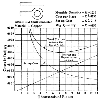
The EOQ problem is stated as Model 1, a special case of the minimum-TLC shipment size model of Lecture 3.3 (Model 1 in Lecture 3.3): each of its differences is a choice of that model’s data, a fixed cost per batch in place of the truckload charge, \alpha set at one half, a payload too large to bind, and a less-than-truckload (LTL) charge too high for LTL ever to be selected.
minimize: total logistics cost of producing, ordering ortransporting a product point-to-point (P2P)periodically, transportfixed cost plus cycle inventory
solve for:
(a) average batch, order orshipment size, a positive weight in tonsor number of units;.
(b) service that carries it, TL or LTL.
subject to:
(a) payload: a TL shipment is no larger than one full truckload;
(b) validity: an LTL shipment stays within the range the LTL rate estimate was fitted on. none
assumptions:
(a) annual demand is known and constant;
(b) product value, carrying rate and inventory fraction do not depend on shipment size;
(c) in-transit inventory is the same for TL and LTLevery size, so it is not a relevant cost.;
(d) each batch, order or shipment arrives all at once, so the inventory fraction is one half.
The total annual logistics cost of batches of size q is that of the truckload model, Eq. 7, with a fixed cost c_o per batch in place of the truckload charge and \alpha = \tfrac{1}{2}:
\min_{q > 0} \; TLC(q) = \frac{f}{q}\, c_o + \frac{1}{2}\, v h q \tag{9}
and setting its derivative with respect to q to zero gives the economic order quantity:
q^{*} = \sqrt{\frac{2 f c_o}{v h}} \tag{10}
where
No Logjam function computes the EOQ, so its implementation is written out here:
Example 4: EOQ for setup costs
A manufacturer produces a replacement part with steady annual demand of 100,000 units. Each production run requires a $250 setup for cleaning, tooling, and inspection. Finished parts are worth $100 each, and holding inventory incurs costs of about 30% of their value per year for capital, storage, and obsolescence. Production is assumed instantaneous, and demand is constant. Determine the optimal number of parts to produce per run to minimize the combined annual cost of setups and inventory.
With steady demand and a setup cost given, the data can be plugged into the formula to solve for q^*, just as for the periodic truckload problem of Lecture 3.3. What was done there for the optimal truckload size is done here more generally, and this is the classic type of EOQ.
Example 4(a): EOQ by hand
With f = 100{,}000 units per year, c_o = \$250 per run, v = \$100 per part and h = 0.3 per year, the total logistics cost of Eq. 9 is a function of the run size q alone:
TLC(q) = \frac{f}{q}\, c_o + \frac{1}{2}\, v h q = \frac{100{,}000}{q}\, 250 + \frac{1}{2}\, 100 (0.3)\, q
Its minimum is at the EOQ of Eq. 10, with the same four values:
q^{*} = \sqrt{\frac{2 f c_o}{v h}} = \sqrt{\frac{2 (100{,}000)\, 250}{100 (0.3)}} \approx 1{,}291 \text{ parts/run}
The Assumptions check of Lecture 1.2 is on the one half in Eq. 9, which holds because production is instantaneous and demand is constant, as the statement assumes. Harris put the condition this way: the average stock is one-half of the lot size if the movement is regular, and if the movement is irregular, as it generally is, an additional complication is introduced.3
q^{*} = 1,291 parts per run
Example 4(b): EOQ in code and by brute force
Determine the number of parts per run with the implementation of Model 1 and by a brute-force search of Eq. 9 over every whole number of parts, and compare both with Ex. 4(a).
Code block 6 enters the data of the statement in the symbols of Eq. 10:
1290.9944487358057A run larger than a year’s demand is never needed, so the search runs from 1 to f parts, evaluating one run size at a time:
totlogcost is the Logjam function of Lecture 3.3 for the total logistics cost of a shipment size; with its \alpha set at one half it is Eq. 9. Each run size is paired with its cost, and minimum compares the pairs by cost first, so it returns the least cost together with its run size, as Code block 4 of Lecture 5.2 does for routes.
(38729.83346243222, 1291)The implementation gives 1,290.99 parts per run, the 1,291 of Ex. 4(a), and the Triangulate check of Lecture 1.2 is that the search, which uses only Eq. 9 and no calculus, finds its minimum at 1,291 parts per run, the EOQ rounded to a whole part.
q^{*} = 1,291 parts per run, at TLC = $38,729.83 per year
Safety stock is held to buffer the effects of uncertainty, and it comes in two kinds. One-time safety stock is the case of uncertain demand and of not being able to carry inventory: unmet demand is a lost sale, excess (expired or obsolete) product is disposed of, and the optimal policy is a trade-off between lost profit and disposal cost. Periodic safety stock is the case of uncertain demand and/or transport lead time and of being able to carry inventory: unmet demand is either a lost sale or a backorder, excess product is carried over to the next period, and the optimal policy is a trade-off with lost profit or backorder cost and inventory carrying cost. Periodic safety stock is the subject of Lecture 6.2.
One-time and periodic safety stock are distinguished just as one-time and periodic truck shipments were, and the periodic case is a little more complicated. Both deal with uncertain demand: if demand were certain, safety stock would never be needed. The important thing for one-time safety stock is that inventory cannot be carried. With daily production, for example, whatever product is left at the end of the day is obsolete, essentially worthless, and cannot be carried over to the next day. This is the classic news vendor problem, named for the idea that nobody wants a day-old newspaper; it is called one-time safety stock here because, although it is essentially the same problem, it is solved differently from the technique most textbooks use. Any unmet demand is a lost sale, so whatever revenue a customer who is not served would have brought is lost, while with periodic safety stock unmet demand can also be backordered, the customer willing to wait a day or two for a product that does not expire in one period. The optimal policy is then the trade-off between lost profit and disposal cost. The disposal cost need not be just what was spent to make the product: a product that cost $5 to make and sells for $10 might be salvaged for $5 at a retailer of odd merchandise, while a hazardous product might cost something to dispose of, so the disposal cost can be positive or negative relative to that.
If the demand d for tomorrow is known, then q = d units should be produced, and the only interesting question is how cheaply the units can be produced. If the demand D for tomorrow is unknown, then how many units q to produce becomes an interesting question. Batch production and consumption can be assumed \Rightarrow IC_{w+e} = 0, and the operating profit if q units are produced and demand turns out to be d_i is:
\begin{aligned} \text{Profit: } & \pi(q, d_{i}) = \begin{cases} p d_{i} - c q , & \text{if } q > d_{i} \\ p q - c q = (p - c) q , & \text{otherwise} \end{cases} \\ & \hphantom{\pi(q, d_{i})} = \boxed{p \min\{q, d_{i}\} - c q} \\[8pt] \text{Lost sales: } & \max\{d_{i} - q, 0\} \\[8pt] \text{Lost profit: } & (p - c) \max\{d_{i} - q, 0\} \end{aligned} \tag{11}
where
Operating profit includes both the cost and the revenue side. If tomorrow’s demand were known, q would simply be set equal to it, and the only question would be how cheaply the units can be produced, a matter of minimizing cost. The capital D indicates that demand is stochastic: it is not known, and how many to produce becomes the interesting question. With batch production and consumption, all of the working and economic inventory goes to zero, so the only reason not to produce the known demand is that the demand is not known.
For any quantity q produced and demand d_i realized, there are two possibilities. If more was produced than the demand, revenue is collected only on the actual demand: with five units sold and ten produced, the revenue is five times the price, but the cost is c times ten units, and the profit that day can very likely be negative. If demand equals or exceeds the quantity produced, the price is received on everything produced: with a demand of 15 and ten produced, five customers are lost sales, and the revenue is for the ten produced, less the cost of producing them. Since q appears in both terms, it can be taken out, leaving p - c, the operating unit profit, the price received less the cost; if the price equaled the cost the profit would be zero, so to be interesting the price has to exceed the cost. The two conditions can be replaced, without an if statement, by the smaller of the quantity produced and the actual demand, times the price, less the cost times the quantity produced: this is the basic news vendor profit equation. Lost sales are positive when demand is greater than the quantity and zero when too much is produced, though then there is product to dispose of, and lost profit is the unit profit times the larger of that difference and zero.
One-time safety stock is a data-rich problem, and the data should be leveraged as much as possible, which is why the standard news vendor approach is not used here. That approach assumes a distribution for demand, such as a Poisson, normal, negative binomial or gamma distribution, which raises the question of how to know which distribution; fitting one to a lot of data and then using only the distribution is like having a room full of great data and throwing it all away for a mathematical substitute. The textbook approach looks for the critical fractile of the cumulative distribution, and there may be some reason to do that, but none has been seen for this problem. The approach taken here, which uses the data directly, is not found in textbooks, so an AI tool would likely say that it cannot be done this way.
When a unit under and a unit over cost the same, the problem is the minisum in one dimension of Lecture 2.1 (Model 8 in Lecture 2.1). Each data point is an existing facility (EF) of weight one, and the solution is their median (Eq. 5 in Lecture 2.1), found by the same procedure. Ex. 5 shows it, with a cost in time rather than profit:
Example 5: Pre-fill level of a test tank
A testing center has a device that is able to use ultrasonic waves transmitted within a special solution to detect defects in parts like aircraft engines. The part is placed in a tank that, in order to operate correctly, is filled with just enough solution to submerge the part; the solution is then drained from the tank and disposed of since it can become contaminated during testing. Currently, test results are being delayed because it is time-consuming to fill the tank with the solution. In order to speed up testing, a suggestion has been made to consider pre-filling the tank and then either adding or draining the solution as needed to submerge a part. The following demand data is available regarding the cubic volume of solution that was needed to test recent parts:237, 214, 161, 146, 331, 159, 423, 332, 139, 327, 152, 98, 116 Determine the cubic volume of solution that should be pre-filled in the tank to minimize the time required to submerge the part, given that the tank can be filled or drained at the same rate.
It is a good idea to look at the data to see if there is a pattern to the data and check to see if there are any anomalous, outlier data that could be erroneous. If anything is found, it might be possible to ask whoever provided the data about the issue before doing any further analysis. If some data is in error, then it can be deleted; outlier data should not automatically be eliminated unless it is a real error.
It is easy to display 1-D, a little harder but doable for 2-D, and difficult for 3+ degree data, where the best that can usually be done is to look at different 1- and 2-D cross-sections of the data. For this data, since there is no time element, a histogram is used instead of a scatter or line plot (Fig. 2).
# Code block 8: the pre-fill demand data and its histogram
d = [237, 214, 161, 146, 331, 159, 423, 332, 139, 327, 152, 98, 116]
fig = Figure(size = (600, 300))
ax = Axis(fig[1, 1]; xlabel = "Demand (cubic volume)", ylabel = "Count",
xlabelsize = 15, ylabelsize = 15,
xticklabelsize = 13, yticklabelsize = 13)
bluec = colorant"#1f6fb5" # data, as in Lectures 4.1 to 5.3
hist!(ax, d; bins = 0:50:450, color = bluec, strokecolor = :white,
strokewidth = 1)
fig
Example 5(a): Pre-fill level by hand
Determine the pre-fill level by hand, as the median of the demands.
Each part is an EF of weight one, so W = 13, and with d_{(j)} the jth smallest demand, in order the demands and their running count are
\def\tight#1{\kern-3pt #1\kern-3pt} \begin{array}{l|ccccccccccccc} d_{(j)} & \tight{98} & \tight{116} & \tight{139} & \tight{146} & \tight{152} & \tight{159} & \tight{\mathbf{161}} & \tight{214} & \tight{237} & \tight{327} & \tight{331} & \tight{332} & \tight{423} \\ j & 1 & 2 & 3 & 4 & 5 & 6 & \mathbf{7} & 8 & 9 & 10 & 11 & 12 & 13 \end{array}
The first j at which the count reaches W/2 = 6.5, as in Eq. 5 in Lecture 2.1, is j = 7, so the pre-fill level is the seventh demand in order, 161.
q^{*} = 161, the median demand
Example 5(b): Pre-fill level in code
Determine the pre-fill level in code by the median procedure of Lecture 2.1, and the level that minimizes the total time numerically, and compare both with Ex. 5(a).
Not seeing anything unusual in the histogram, the next step can be to develop a model that captures the “cost” of different pre-fill levels, where the cost, in this case, can be the time required to either fill or drain the tank from the pre-fill level, where it is assumed that, for a given volume of solution, the fill and drain times are the same since their rates are the same, and the time to fill or drain the tank from the pre-fill level for each part is
\text{Time: } t(q, d_i) = \bigl| d_i - q \bigr| \tag{12}
where
A unit under and a unit over take the same time, so the median procedure of Lecture 2.1 applies unchanged, in the code Lecture 2.2 gave it (Ex. 1(b) in Lecture 2.2): sort the demands, give each part a weight of one, and stop at the first part whose running total of weight reaches half the total. Code block 9 runs it first, then minimizes the total time of Eq. 12 over the 13 parts by brute force and numerically, and Fig. 3 draws the total time against the pre-fill level, with the minimum the search finds in maroon:
# Code block 9: pre-fill level by the median procedure, then numerically
# the median procedure of Lecture 2.1, as Lecture 2.2 coded it
ds = sort(d) # demands in order
w = ones(Int, length(ds)) # each part an EF, weight one
@show W = sum(w)
@show j = findfirst(>=(W / 2), cumsum(w)) # first running total >= W/2
@show qmed = ds[j]
# the total time over the 13 parts, minimized
using Optim
ft(q, di) = abs(di - q) # time for a single part
fTT(q, d) = sum(ft(q, di) for di in d) # total time
# brute force first: each whole-number level, one at a time
TTmin, qmin = minimum((fTT(q, d), q) for q ∈ 0:maximum(d))
@show qmin
qᵒ = optimize(q -> fTT(q, d), 0, maximum(d)).minimizer
@show round(qᵒ, digits = 2)
@show round(fTT(qᵒ, d), digits = 2);W = sum(w) = 13
j = findfirst((>=)(W / 2), cumsum(w)) = 7
qmed = ds[j] = 161
qmin = 161
round(qᵒ, digits = 2) = 161.0
round(fTT(qᵒ, d), digits = 2) = 1054.0# Code block 10: total time against the pre-fill level
fig = Figure(size = (600, 320))
ax = Axis(fig[1, 1]; xlabel = "Pre-fill level", ylabel = "Total time",
xlabelsize = 15, ylabelsize = 15,
xticklabelsize = 13, yticklabelsize = 13)
optc = colorant"#b23a48" # an optimum, as in Lecture 2.2
lines!(ax, 0:maximum(d), q -> fTT(q, d); color = bluec, linewidth = 2)
scatter!(ax, [qᵒ], [fTT(qᵒ, d)]; color = optc, markersize = 13)
fig
The Landmark check of Lecture 1.2 is that the numerical minimum, at 161, is the median found by hand in Ex. 5(a) and by the procedure in Code block 9, an answer known before the search was run.
q^{*} = 161, at a total time of 1054
Example 5(c): Extreme outlier
Determine the pre-fill level if the demand of 423 had instead been 1,423.
Since the solution is only as good as the model and data used to generate it, it is helpful to try to determine how robust the solution is with respect to the data that was used and the assumptions behind the model. Starting with data robustness, one thing that can be checked is what if there had been an extreme outlier in the data. For example, if the 423 demand was instead 1,423, would the solution change significantly?
# Code block 11: the pre-fill level with an extreme outlier
d2 = copy(d) # a copy: d2 = d would only point to d, and
d2[d2 .== 423] .= 1423 # a change to d2 would also change d
qᵒ2 = optimize(q -> fTT(q, d2), 0, maximum(d2)).minimizer
@show round(qᵒ2, digits = 2)
@show round(fTT(qᵒ2, d2), digits = 2);round(qᵒ2, digits = 2) = 161.0
round(fTT(qᵒ2, d2), digits = 2) = 2054.0Although, as expected, the total time increases by 1,000, it might seem surprising that the optimal pre-fill level remains unchanged. The reason for this is, for this particular objective function, the optimal solution is the value of the median demand point. Any unit increase in the solution would increase by one unit the times of all of the demands less and decrease by one unit the times of all demands greater than the solution. Since the unit cost of filling and draining are the same and, being the median point, there are equal numbers of points less than and greater than the solution, the optimal solution remains unchanged. This is Lecture 2.1’s argument for the median location, and its result as well: moving Asheville, the westernmost of the cities on I-40, all the way to California leaves the minisum location where it was, since the median procedure uses only the order of the facilities, never their coordinates (Fig. 7 in Lecture 2.1). Raising the largest demand from 423 to 1,423 is the same move, the last point on the line taken farther out with the order unchanged.
median(d) = 161.0
median(d2) = 161.0q^{*} = 161, unchanged, at a total time of 2054
When a unit under and a unit over cost different amounts, as filling and draining do in Ex. 5(d), which follows, and as a lost sale and a disposed unit do, the quantity is the one that minimizes the total overage and underage cost over the demand history, stated as Model 2, a generalization of the minisum in one dimension of Lecture 2.1 (Model 8 in Lecture 2.1), and formulated as Eq. 13. That minisum, with each EF of weight one, is its special case: with c_{\text{over}} = c_{\text{under}}, a unit under and a unit over cost the same, and minimizing the total cost is minimizing the total of \lvert d_i - q \rvert, as in Ex. 5(a) to (c), the demands the EFs and the quantity the location of the new facility. Ex. 5(d) is the case c_{\text{over}} = 1 and c_{\text{under}} = 2, a unit drained taking half the time of a unit filled.
minimize: total weighted distance from a new facility (NF) to the m existing facilities (EFs) along a lineoverage and underage cost over the demand history, when the same quantity is set for each demand before that demand is known
solve for:
(a) location x of the NF, any point along the linequantity set for each demand, the same for every demand.
subject to: none
assumptions:
(a) facilities lie on a single line, so distance is one-dimensional; a two-dimensional problem with rectilinear distance is solved by applying the model once along each axisdemand is stationary, so the history represents the variability of any one demand;
(b) each EF’s weight w_i is known, and the EFs can be placed in order along the line, but their actual coordinates are not neededoverage cost of a unit over and underage cost of a unit under are constant;
(c) inventory cannot be carried from one demand to the next.
With an overage cost c_{\text{over}} for each unit the quantity exceeds a demand and an underage cost c_{\text{under}} for each unit a demand exceeds the quantity, the quantity solves
\min_{q \ge 0} \; C(q) = \sum_{i=1}^{N} \Bigl[\, c_{\text{over}} \max\{q - d_i, 0\} + c_{\text{under}} \max\{d_i - q, 0\} \,\Bigr] \tag{13}
where
No Logjam function computes it, so its implementation is written out here:
mincost (generic function with 1 method)Example 5(d): Filling twice as slow as draining
Determine the pre-fill level if the drain rate is twice the fill rate, for the demands with and without the outlier.
The assumption in the model that is most questionable is assuming that the fill and drain rates are the same; this would only be true if the diameters of the fill and drain tubes are the same along with the flow rates being the same. If, after further investigation, it was found that the drain rate was twice the fill rate, then the model can be modified to incorporate this. Since the “cost” of filling and draining is now unbalanced, with filling taking twice as long as draining, the median point will not, in general, correspond to the optimal solution, and the cost of the pre-fill level for each part, in time, becomes
\text{Pre-fill cost: } c(q, d_i) = \begin{cases} 2(d_i - q), & \text{if } d_i > q \\ q - d_i, & \text{otherwise} \end{cases} \tag{14}
where
The total of Eq. 14 over the parts, Eq. 13 with c_{\text{over}} = 1 and c_{\text{under}} = 2, is minimized for each data set by the implementation of Model 2:
(237, 237)At the level of 237 found with the demands as given, the 8 smaller parts are drained, 711 units in all, and the 4 larger ones filled, 465 units, so by Eq. 13 the total time is
\begin{aligned} C(237) &= c_{\text{over}} \sum_{i=1}^{N} \max\{237 - d_i, 0\} + c_{\text{under}} \sum_{i=1}^{N} \max\{d_i - 237, 0\} \\ &= 1(711) + 2(465) = 1{,}641 \end{aligned}
As expected, since it is more costly to fill than to drain, the optimal pre-fill level has increased and is no longer the median but is still robust with respect to data outliers; that the level moved the way the change in costs predicts is the Nudge check of Lecture 1.2.
q^{*} = 237 with the demands as given and 237 with the outlier
For a product made each day and sold at a unit price, as in Eq. 11, a unit over costs the unit cost, c_{\text{over}} = c, since it is made and not sold, and a unit under costs the operating unit profit, c_{\text{under}} = p - c, the profit of the lost sale. With perfect prediction, the number made each day exactly matches that day’s demand, so no unit is over or under, and the unit profit is made on every unit of demand. The total operating profit over the history is then the total operating profit of perfect prediction less the overage and underage cost:
\hphantom{\underset{\displaystyle \Pi^{UB}}{\Pi(q)}}\mathllap{\Pi(q)} = \mathrlap{\sum_{i=1}^{N} \Bigl[\, p \min\{q, d_i\} - c q \,\Bigr] = \Pi^{UB} - C(q)}\hphantom{\underset{\displaystyle (p - c) \sum_{i=1}^{N} d_i}{\sum_{i=1}^{N} \Bigl[\, p \min\{q, d_i\} - c q \,\Bigr] = \Pi^{UB} - C(q)}} \tag{15}
\hphantom{\underset{\displaystyle \Pi^{UB}}{\Pi(q)}}\mathllap{\Pi^{UB}} = \mathrlap{(p - c) \sum_{i=1}^{N} d_i}\hphantom{\underset{\displaystyle (p - c) \sum_{i=1}^{N} d_i}{\sum_{i=1}^{N} \Bigl[\, p \min\{q, d_i\} - c q \,\Bigr] = \Pi^{UB} - C(q)}} \tag{16}
where
so the quantity that minimizes C(q) is the one that maximizes \Pi(q). A salvage value or a cost of disposal, as discussed at the start of Sec. 4, changes only c_{\text{over}}.
Model 2 is the classic newsboy, or news vendor, problem4: each morning a newsboy buys the day’s papers before knowing how many will sell, a paper under is a sale lost, and a paper over is worth nothing the next day. The name is not used here for three reasons. It names one application, and the model serves others in which nothing is sold, the pre-fill level of Ex. 5 and, at the end of this section, the time ahead to order an item whose lead time is uncertain; one-time names what they all share, that nothing over can be carried to the next demand, which is what separates them from the periodic safety stock of Lecture 6.2. And the name comes with a way of solving the problem, the fitted distribution and its critical fractile described under Operating profit. Here, instead, the total cost of Eq. 13 is minimized on the history itself, by brute force or with an optimizer, so no distribution has to be chosen and every demand of the history is used.
Third, and most important, minimizing on the history carries over unchanged when the quantity is allowed to change from day to day with what is known that morning. Starting with the morning’s orders, and then expanding to include the website’s visitors, Ex. 6 makes them the independent variables of a multiple linear regression, Model 3, and that regression formulation is the starting point for machine learning. The basic idea is that, instead of just a point estimate, the same quantity for every demand, any additional data that is in some way correlated with the decision allows more information to be used in making it. Ex. 6 uses just two data sources, where classic machine learning techniques use dozens, if not hundreds. Machine learning is not covered in this course, but this is its starting point, and the example that follows illustrates its benefits.
Example 6: Lee Pharm’s bakery
Lee Pharm owns a bakery and has to determine each morning how many loaves of bread to bake for the day. Any loaves unsold at the end of the day are donated to the local homeless shelter. He would like some help with how to best determine the number of loaves to bake each day. He has available the number of loaves sold for each of the last 13 days:
216, 214, 161, 146, 216, 159, 216, 216, 139, 216, 152, 98, 116
In looking at the data, the first thing noticeable is that the number 216 appears quite often. After talking with Lee, it turns out that he typically makes 216 loaves per day, which corresponds to 18 trays of a dozen loaves. Since there was likely unmet demand any day that 216 loaves were sold, after checking with Lee, it turns out that he also has been recording the number of customers asking for bread each day after it was sold out. After adding in this unmet demand, the adjusted potential demand is:
237, 214, 161, 146, 331, 159, 423, 332, 139, 327, 152, 98, 116
After confirming with Lee that these past 13 days of demand are reasonably representative of typical demand, the only other information needed to provide some guidance is the average selling price of each loaf and the cost to bake each loaf, which turns out to be $5 and $1, respectively. Also, Lee agrees that it is reasonable to assume that any demand for a day that is not filled is lost; this is because most customers consume their bread the day of purchase, since it is made without preservatives. Determine the number of loaves to bake each day that maximizes total profit.
Example 6(a): Stationarity of the demand
Determine whether the 13 days of demand can be taken as stationary.
Before analysis, review the data for unusual values and overall patterns. Confirm questionable points with the source and remove only clear errors, not outliers by default. Also check whether the data appear stationary, since nonstationary series require detrending or other adjustments. A line plot is used because the 13 days of demand represent a time series.
Fig. 4(a) shows no trend or seasonality that would need to be accounted for in any model of the data. Most importantly, the variability does not show a long-term pattern and so it is assumed that the data is stationary. There are statistical tests for stationarity, but these would not typically be used for so few data points. Since stationarity implies the lack of trend/seasonality, the data can be randomly re-arranged (or permuted), and it should look about the same. This is done in Fig. 4(b) and (c) to verify stationarity, an Assumptions check of Lecture 1.2.
Code block 14 draws the three panels with a helper function, plotperms, so that the same check can be made on any other series by a single call. Its settings are collected at its top, and adapting the plot means changing only those. The seed of its random permutations is an optional keyword argument, 2523 unless a call gives another:
# Code block 14: a helper that plots a series as observed and in two
# random permutations, used on the bakery's demand
using Random
function plotperms(x, ylabel, caption_a; seed = 2523)
# settings: change these to adapt the plot
figsize = (600, 560) # width and height, pixels
color = bluec # color of the line
arrowc = :gray40 # color of the arrows from (a)
sizes = (xlabelsize = 15, ylabelsize = 15,
xticklabelsize = 13, yticklabelsize = 13)
captions = (caption_a, "a random permutation", "a random permutation")
# the plot: one panel per order, each captioned below
N = length(x) # number of values in the series
Random.seed!(seed) # the same permutations every run
orders = (1:N, randperm(N), randperm(N))
fig = Figure(size = figsize)
axs = [Axis(fig[2k - 1, 1]; ylabel, xticks = 1:N, sizes...)
for k in 1:3]
for k in 1:3
lines!(axs[k], 1:N, x[orders[k]]; color, linewidth = 2)
Label(fig[2k, 1], "($('a' + k - 1)) $(captions[k])";
fontsize = 15, tellwidth = false)
end
# an arrow from (a) to each panel derived from it, at their right
colsize!(fig.layout, 1, Relative(0.92))
vp = [ax.scene.viewport[] for ax in axs]
xr = vp[1].origin[1] + vp[1].widths[1] # panels' right edge
ym = [v.origin[2] + v.widths[2]/2 for v in vp] # their middles
lines!(fig.scene, [xr + 4, xr + 22, xr + 22], [ym[1], ym[1], ym[3]];
color = arrowc, linewidth = 1.5)
arrows2d!(fig.scene, fill(xr + 22, 2), ym[2:3], [-18, -18], [0, 0];
color = arrowc)
return fig
end
d = [237, 214, 161, 146, 331, 159, 423, 332, 139, 327, 152, 98, 116]
plotperms(d, "Demand", "day by day")seed is, is optional: a call that leaves it out gets 2523, and plotperms(d, "Demand", "day by day"; seed = 1) draws two other permutations.
sizes... in the call to Axis passes each of them as a keyword argument of the same name.
1:N, is the series as observed. randperm(N) is a random reordering of the numbers 1 to N, so indexing the series by it, as x[orders[k]] does in the call to lines!, permutes the series.
ylabel is here and color is in the call to lines!, passes the variable of that name as the keyword argument of the same name, so the axis label is the function’s second argument.
k sits in row 2k - 1 of the figure’s grid and its caption in row 2k, below it; 'a' + k - 1 is the letter a, b or c.
viewport gives each one’s place on the figure, in pixels from its lower left corner, so the arrows are drawn on the figure itself, fig.scene, rather than in a panel: a line from the right of (a) down to the middle of (c), with an arrowhead into (b) and into (c), the two panels derived from (a). colsize! keeps the panels to 92% of the width, leaving room for the arrows.

The two plots of a random permutation of the demands also look stationary, lacking trend/seasonality.
The demand can be taken as stationary.
Example 6(b): Baseline and upper bound
Determine the total profit of baking 216 loaves each day, and an upper bound on total profit.
In order to be able to compare the effectiveness of any procedure, a baseline and upper bound on total profit can be determined. The baseline is the total profit associated with using the current practice of baking 216 loaves per day. An upper bound can be determined by assuming that the number of loaves baked each day exactly matches that day’s demand (perfect prediction).
Perfect prediction makes the unit profit on every unit of demand, and the total demand is the mean scaled up by the number of days, as in Lecture 1.1:
\bar{d} = \frac{\sum_{i = 1}^{N} d_{i}}{N} \Rightarrow N \bar{d} = \sum_{i = 1}^{N} d_{i}
With the unit price of $5 and unit cost of $1, the upper bound on total profit over the 13 days is then
\Pi^{UB} = (p - c) \sum_{i=1}^{N} d_i = (p - c)\, N \bar{d} = (5 - 1)(2{,}835) = 11{,}340
and by Eq. 15, with c_{\text{over}} = c = 1 and c_{\text{under}} = p - c = 4, baking 216 loaves every day leaves 543 loaves over on the 8 days of lower demand and 570 under on the other 5, so the baseline is
\begin{aligned} \Pi(216) &= \Pi^{UB} - C(216) = 11{,}340 - \bigl[\,1(543) + 4(570)\,\bigr] \\ &= 11{,}340 - 2{,}823 = 8{,}517 \end{aligned}
With the same unit price and cost, c_{\text{over}} = c and c_{\text{under}} = p - c, and the total profit of Eq. 15, the upper bound of Eq. 16 less the total cost of Model 2’s implementation, gives the baseline:
# Code block 15: baseline and upper bound on total profit
p = 5 # $/loaf, unit price
c = 1 # $/loaf, unit cost
c_over = c # $/loaf over: baked and not sold
c_under = p - c # $/loaf under: the profit lost
fΠ(q, d) = (p - c)*sum(d) - fC(q, d) # total profit: bound less cost
Πᴮᴸ = fΠ(216, d) # baseline: 216 loaves every day
Πᵁᴮ = (p - c)*sum(d) # upper bound: perfect prediction
@show Πᴮᴸ
@show Πᵁᴮ
@show Πᴮᴸ/Πᵁᴮ;Πᴮᴸ = 8517
Πᵁᴮ = 11340
Πᴮᴸ / Πᵁᴮ = 0.7510582010582011Baseline $8,517, upper bound $11,340, the baseline 75% of it
Example 6(c): Maximum total profit
Determine the number of loaves to bake each day that maximizes total profit, by brute force, and check it with a numerical optimizer.
Since the demand data is assumed stationary, no attempt is made to predict each day’s demand; instead, the historical demand data is taken as representative of the variability of any day’s demand, as a result, all of the data is used to determine the same (optimal) number of loaves to bake each day. Note: the numerical optimizer uses 500 as the upper bound (UB) for its search since it is likely that daily demand might exceed the maximum (423) found using just the 13 days of data.
The brute force of Model 2’s implementation evaluates the total cost of Eq. 13 at every whole number of loaves from none to the largest demand, and by Eq. 15 the least total cost is the greatest total profit:
qᵒ = 331
Πᵒ = 9407
Πᵒ / Πᵁᴮ = 0.8295414462081129
Πᵒ / Πᴮᴸ = 1.1044968885757895and the numerical optimizer searches the interval from 0 to 500:
round(qᵒOptim, digits = 2) = 331.0
round(fΠ(qᵒOptim, d), digits = 2) = 9407.0# Code block 18: total profit against the loaves baked each day
fig = Figure(size = (600, 320))
ax = Axis(fig[1, 1]; xlabel = "Loaves baked each day",
ylabel = "Total profit (\$)", xlabelsize = 15, ylabelsize = 15,
xticklabelsize = 13, yticklabelsize = 13)
lines!(ax, 0:500, q -> fΠ(q, d); color = bluec, linewidth = 2)
scatter!(ax, [qᵒ], [Πᵒ]; color = optc, markersize = 13)
fig
The Triangulate check of Lecture 1.2 is that the brute force and the optimizer, two different methods, find the same 331 loaves (Fig. 5, the maximum in maroon). The solution recommends that Lee bake 331 loaves each morning, which should result in an over 10% increase in total profits as compared to baking only 216 loaves. The procedure works because the data is stationary, lacking trend/seasonality. If the data has a trend/seasonality, techniques exist that can try to remove the trend/seasonality so that all of the data can be used; otherwise, for non-stationary data, only the most recent data would be used in any estimate. If, for example, sales have significantly increased in the past week and are expected to remain at this higher level for at least the next few days, then the nonlinear optimization could be rerun using just the last week’s data.
q^{*} = 331 loaves, at a total profit of $9,407
Example 6(d): Mean, median and safety stock
Determine the total profit of baking the mean and the median demand each day, and the safety stock of the maximum-profit number of loaves.
Mean and Median: By way of comparison, what if the mean or median values for demand were used to determine the number of loaves to bake each morning:
mean(d) = 218.07692307692307
fΠ(mean(d), d) = 8541.923076923078
median(d) = 161.0
fΠ(median(d), d) = 7592.0After checking with Lee, the fact that the mean value of 218 is close to the 216 loaf value he was using is no accident: it turns out that he averaged an earlier set of historical demand values to determine the 216 value. Lee had arrived at 216 by looking at the average demand over some earlier period, around 218. The reason 216 was picked instead of the mean, 218, is that 216 is 18 dozen, and his baking pans are for a dozen, so he rounds to dozens for convenience. The obvious thing, producing the demand that is expected, does not work here, and the median is even worse; the reason 331 does better than 218 is what is called asymmetric loss. The mean assumes symmetric loss: it weights above and below equally, and so does the middle thing. If the problem were to estimate what demand will be, 218 would be a better number than 331, and 331 is not a prediction of demand. Because demand is not perfectly predictable, it is better to produce 331, since there is more upside than downside: every extra customer who walks in above the average gains $4 in net profit, and every loaf produced and not needed loses $1, a four-to-one trade-off. That asymmetry makes the problem different from estimating demand: the goal is to maximize total profit, not to minimize the squared error loss that the average minimizes.
When losses are symmetric, like in the pre-fill of Ex. 5, two different objectives can be used to estimate parameter(s) \hat{y} in a model given data y:
\begin{aligned} \text{L1 loss: } \sum \bigl| \hat{y} - y \bigr| &\implies \text{Minimum Absolute} \\ &\phantom{\implies{}} \text{Deviation (MAD)} \implies \text{Median} \\ \text{L2 loss: } \sum (\hat{y} - y)^2 &\implies \text{Minimum Square} \\ &\phantom{\implies{}} \text{Error (MSE)} \implies \text{Mean} \end{aligned} \tag{17}
Neither loss in Eq. 17 is the bakery’s. Total profit is a nonlinear function of demand, through the minimum in Eq. 11, so by the working rule of Lecture 1.1 the mean demand cannot stand in for the data, and the median, as Lecture 2.5 put it of a minisum location, is the answer to a different question.
There was no safety stock associated with using the mean. Safety stock with lost sales is the units produced in excess of the mean demand. For example, if no penalty backordering was possible, excess production on days of low demand could be held, as economic (anticipation) stock, to satisfy demand on days of under-production. See Lecture 1.1, Sec. 6, on why and when the mean is useful. For the bakery, the safety stock is
\bar{q}_{SS} = q^{*} - \bar{d} = 331 - 218.08 = 112.92 \approx 113 \text{ loaves}
where
Mean 218.08 loaves at $8,541.92, median 161 at $7,592, and a safety stock of 113 loaves at q^{*}
Example 6(e): Loaves by hand
Determine the number of loaves to bake each day by hand, from the demands in order.
The median procedure of Lecture 2.1, used for the pre-fill level in Ex. 5(a), solves the bakery’s problem with one change. As in Ex. 5, the line is measured in units of demand, here loaves. Each day is an EF of physical weight one, located on the line at its demand, and the number of loaves baked, q, is the new facility on the same line. The distance from q to a day’s demand is then the number of loaves over or under that day.
The change is in the transport rate. A monetary weight is a physical weight times a transport rate (Eq. 2 in Lecture 2.2). If the rate were the same in both directions, it could be set to one, as in Lecture 2.2, Sec. 1, making each monetary weight equal to its physical weight of one, and q would be the median, 161, as in Ex. 5(a). For the bakery, the rate depends on the direction of travel. A day whose demand is above q is under, and it travels west to q at $4 a loaf, the unit profit lost, c_{\text{under}} = p - c. A day whose demand is below q is over, and it travels east to q at $1 a loaf, the unit cost of a loaf not sold, c_{\text{over}} = c. Traveling west costs four times as much as traveling east, and the total transport cost is the total overage and underage cost of Eq. 13.
The median argument carries over. If j of the 13 days have demand at or below q, moving q one loaf east adds a loaf of eastward travel to each of those j days, at $1 each, and removes a loaf of westward travel from each of the other 13 - j days, at $4 each. The move lowers the total cost as long as j < 4(13 - j), or 5j < 52, that is, j < 10.4 = 4/5 \times 13, so q keeps moving east until the days at or below it are at least 4/5 of the days. With equal rates, the same argument stops where the days at or below q are at least as many as those above, half of them, which is the median.
The procedure is then that of Ex. 5(a), stopping at 4/5 instead of half: sort the demands, count up from the smallest, and stop at the first j at which the count reaches 4/5 \times 13 = 10.4:
\def\tight#1{\kern-3pt #1\kern-3pt} \begin{array}{l|ccccccccccccc} d_{(j)} & \tight{98} & \tight{116} & \tight{139} & \tight{146} & \tight{152} & \tight{159} & \tight{161} & \tight{214} & \tight{237} & \tight{327} & \tight{\mathbf{331}} & \tight{332} & \tight{423} \\ j & 1 & 2 & 3 & 4 & 5 & 6 & 7 & 8 & 9 & 10 & \mathbf{11} & 12 & 13 \end{array}
so j = 11, and 331 loaves are baked each day, as the brute force of Code block 16 found. As with the median, only the order of the demands determines which one is chosen, not the distances between them, just as the mile markers never entered Ex. 1(b) in Lecture 2.2.
In general, the count stops at the fraction c_{\text{under}}/(c_{\text{over}} + c_{\text{under}}) of the days, the westward rate’s share of the two rates. With equal rates the fraction is 1/2, the median of Ex. 5(a), and with the westward rate of 2 and eastward rate of 1 of Ex. 5(d) it is 2/3, the ninth demand in order, 237.
q^{*} = 331 loaves, the eleventh demand in order
When information that arrives each morning, such as preorders, is related to that day’s demand, the number produced can differ from day to day as a function of it, and Model 2 becomes Model 3, a generalization in which the number produced each day is a linear function of one or more independent variables known that morning, a multiple linear regression. Model 2 is the special case with no independent variables, in which the intercept alone is produced every day. One model then serves for any choice of the independent variables, the morning’s orders alone in Ex. 6(f) and the orders and the website’s visitors together in Ex. 6(g), where a model for each choice would otherwise be needed.
minimize: total overage and underage cost over the demand history, when the same quantity is set for each demand before that demand is knownthe quantity set for each demand before it is known is a linear function of the independent variables known by then, its intercept and coefficients chosen once for all demands
solve for:
(a) quantity set for each demand, the same for every demandintercept and coefficients of the production rule.
subject to: none
assumptions:
(a) relation between the independent variables anddemand is stationary, so the history represents the variability of any one demand;
(b) overage cost of a unit over and underage cost of a unit under are constant;
(c) inventory cannot be carried from one demand to the next.
The quantity set for each demand follows the production rule, a linear function of the m independent variables known before it is set,
\hat{q}_i = a_1 + a_2 x_{i1} + \cdots + a_{m+1} x_{im} = a_1 + \sum_{j=1}^{m} a_{j+1} x_{ij} \tag{18}
and with the overage and underage cost of Eq. 13 on each demand of the history, the intercept and coefficients of the production rule, Eq. 18, solve
\begin{aligned} \min_{a_1, \ldots, a_{m+1}} \; C(a_1, \ldots, a_{m+1}) = \sum_{i=1}^{N} \Bigl[\, & c_{\text{over}} \max\{\hat{q}_i - d_i, 0\} \\ & + c_{\text{under}} \max\{d_i - \hat{q}_i, 0\} \,\Bigr] \end{aligned} \tag{19}
where
Its implementation is three definitions, one for each piece of the formulation: the total cost of Eq. 19 when the quantity differs from one demand to the next, the production rule of Eq. 18, and mincost, which finds the intercept and coefficients that minimize that total cost. Each independent variable is a vector with one value for each demand, and any number of them can follow the demand, so mincost(d, o) fits the rule on the orders alone and mincost(d, o, v) on the orders and the visitors together:
q::AbstractVector makes this a second method of fC, which Julia uses only when q is a vector, one quantity for each demand; when q is a single number it still uses the method of Model 2. The dot in fc.(q, d) applies fc to each demand in turn, with its own quantity, and sum adds their costs.
x... in a definition gathers every argument after a, however many there are, into one tuple named x, so x[j] is independent variable j and length(x) is m: fq̂(a, o) has m = 1 and fq̂(a, o, v) has m = 2. Each x[j] is a vector over the days, so the sum is too, and the dot in .+ adds the intercept to each of its elements, giving one size for each day; given single numbers, as in fq̂(a, 120, 45), the rule gives one size.
x... in a call does the reverse of x... in a definition: it spreads the tuple back out into separate arguments, so fq̂(a, x...) is fq̂(a, o) when mincost was called as mincost(d, o). optimize minimizes, so the total cost is handed to it as it is, where the total profit of Code block 17 had to be negated.
optimize searches over all the elements of a together. [0; ones(length(x))] starts the intercept at 0 and each of the m coefficients at 1, which for the orders alone is the rule of baking just the orders, and .minimizer is the a at which the search ends.
mincost (generic function with 2 methods)Example 6(f): Loaves from the morning’s orders
Determine the linear rule on each morning’s orders that maximizes total profit, and compare its total profit with those of the rules fitted by least squares and by least absolute deviation.
Lee is quite pleased with the prospect of a 10% increase in profits and happens to mention that a large number of his customers preorder their purchases and that the number of orders that he has received each morning seems positively correlated with the number of sales he sees that day. He provides the number of orders available each morning for the past 13 days:
121, 143, 63, 80, 198, 52, 160, 162, 85, 106, 129, 141, 106
During each day, additional walk-in demand occurs, and some orders are canceled; as a result, the final demand at the end of the day differs from the amount ordered at the start of the day. Nevertheless, it is thought that using each day’s preorders to help determine the number of loaves to bake that day can increase total profits.
The correlation of the two time series can be calculated, and the two plotted (Fig. 6), to see how likely the order data may help in estimating demand:
# Code block 20: the morning's orders and their correlation with demand
o = [121, 143, 63, 80, 198, 52, 160, 162, 85, 106, 129, 141, 106]
@show cor(o, d)
dcc = colorant"#1e8a3c" # as in Lectures 4.1 to 5.3
fig = Figure(size = (600, 640))
ax1 = Axis(fig[1, 1]; xlabel = "Day", ylabel = "Loaves",
xticks = 1:length(d), xlabelsize = 15, ylabelsize = 15,
xticklabelsize = 13, yticklabelsize = 13)
Label(fig[2, 1], "(a) day by day"; fontsize = 15,
tellwidth = false) # caption, below its panel
lines!(ax1, 1:length(o), o; color = dcc, linewidth = 2,
label = "Orders")
lines!(ax1, 1:length(d), d; color = bluec, linewidth = 2,
label = "Demand")
axislegend(ax1; position = :lt, labelsize = 13)
ax2 = Axis(fig[3, 1]; xlabel = "Orders by the morning",
ylabel = "Demand",
title = "correlation $(round(cor(o, d), digits = 2))",
titlesize = 15, titlefont = :regular, xlabelsize = 15,
ylabelsize = 15, xticklabelsize = 13, yticklabelsize = 13)
Label(fig[4, 1], "(b) demand against orders"; fontsize = 15,
tellwidth = false) # caption, below its panel
scatter!(ax2, o, d; color = bluec, markersize = 10)
figcor(o, d) = 0.5994685344117657
An almost 60% correlation is promising, and so it is likely to be beneficial to include the order data in the analysis. This can be done through linear regression by making the demand a function of order data.
Profit using just order data: What if just the number of orders received by each morning were used to determine the number of loaves to bake that day:
With the orders as its one independent variable, m = 1 and x_{i1} = o_i, Model 3 is specialized to the orders, and its production rule, Eq. 18, becomes
\hat{q}_i = a_1 + a_2 o_i
where
With this rule, the intercept and coefficient that minimize the total cost of Eq. 19 with the bakery’s overage and underage costs are, by Eq. 15, those that solve
\max_{a_1, a_2} \; \Pi(a_1, a_2) = \sum_{i=1}^{N} \Bigl[\, p \min\{\hat{q}_i, d_i\} - c\, \hat{q}_i \,\Bigr]
Code block 22 passes the orders to mincost after the demand, and so fits a linear regression on the orders with profit maximization as the objective:
aΠᵒ = [77.21818171600432, 1.5727272746809993]
fΠ(fq̂(aΠᵒ, o), d) = 9853.636363517973
fΠ(fq̂(aΠᵒ, o), d) / Πᵁᴮ = 0.8689273689169289
fΠ(fq̂(aΠᵒ, o), d) / Πᴮᴸ = 1.1569374619605464Regression as it is usually done fits the rule to demand rather than to profit, by least squares, the L2 loss of Eq. 17, or by least absolute deviation, the L1 loss, and each rule is then judged by its total profit:
fΠ(fq̂(aL2, o), d) = 9326.541533261548
fΠ(fq̂(aL1, o), d) = 9602.259258268658# Code block 24: demand against orders, with the three fitted rules
fig = Figure(size = (600, 380))
ax = Axis(fig[1, 1]; xlabel = "Orders by the morning",
ylabel = "Demand", xlabelsize = 15, ylabelsize = 15,
xticklabelsize = 13, yticklabelsize = 13)
scatter!(ax, o, d; color = bluec, markersize = 10)
x = [0, maximum(o)]
dcc = colorant"#1e8a3c" # as in Lectures 4.1 to 5.3
orc = colorant"#e08214" # as in Lecture 4.2
Πlab(a) = "\$$(commas(round(Int, fΠ(fq̂(a, o), d))))" # its total profit
lines!(ax, x, fq̂(aΠᵒ, x); color = optc, linewidth = 2,
label = "Maximum profit, $(Πlab(aΠᵒ))")
lines!(ax, x, fq̂(aL2, x); color = dcc, linewidth = 2, linestyle = :dash,
label = "Least squares, $(Πlab(aL2))")
lines!(ax, x, fq̂(aL1, x); color = orc, linewidth = 2, linestyle = :dot,
label = "Least absolute deviation, $(Πlab(aL1))")
axislegend(ax; position = :lt, labelsize = 13)
fig
Over the range of orders observed, the rule that maximizes total profit lies above the other two (Fig. 7), for the same reason the size of Ex. 6(c) lies above the mean. For day 14, with 120 loaves ordered by the morning, it bakes
\hat{q}_i = 77.22 + 1.57 o_i, at a total profit of $9,853.64, against $9,326.54 by least squares and $9,602.26 by least absolute deviation; 266 loaves on day 14
Example 6(g): Adding the website’s visitors
Determine the rule on each morning’s orders and the past day’s website visitors that maximizes total profit, and the loaves it bakes on day 14, with 120 orders and 45 visitors.
After further discussion, Lee mentions that he can also access each morning the number of unique visitors to his bakery’s website over the past day, and over the 13 days of the history they were69, 72, 56, 72, 82, 80, 72, 64, 50, 65, 49, 51, 66 Whether this additional data can help is seen from its correlation with demand, and from a plot of the two (Fig. 8):
# Code block 26: the website's unique visitors and their correlation
v = [69, 72, 56, 72, 82, 80, 72, 64, 50, 65, 49, 51, 66]
@show cor(v, d)
fig = Figure(size = (600, 340))
ax = Axis(fig[1, 1]; xlabel = "Unique visitors over the past day",
ylabel = "Demand",
title = "correlation $(round(cor(v, d), digits = 2))",
titlesize = 15, titlefont = :regular, xlabelsize = 15,
ylabelsize = 15, xticklabelsize = 13, yticklabelsize = 13)
scatter!(ax, v, d; color = bluec, markersize = 10)
figcor(v, d) = 0.46082474901378706
A 46% correlation indicates a moderate relationship that may help. In order to effectively use the visitor data, it can be added to the model along with the order data in a multiple regression:
\hat{q}_i = a_1 + a_2 o_i + a_3 v_i
where
This is the production rule of Model 3 with m = 2 independent variables, x_{i1} = o_i and x_{i2} = v_i, and nothing else in Eq. 19 changes, so Code block 27 solves it with the same mincost, the visitors passed after the orders:
aΠᴹᵒ = [0.015104509015262729, 1.6444684204385456, 1.0247033027779333]
fΠ(fq̂(aΠᴹᵒ, o, v), d) = 9902.722869055702For day 14, with 120 orders and 45 visitors:
243.46296358664773Total profit $9,902.72; 243 loaves on day 14
Table 2 sets the total profit of every procedure in Ex. 6 side by side:
# Code block 29: total profit of each procedure
procs = ["Baseline, 216 loaves", "Mean demand", "Median demand",
"Maximum profit", "Orders alone", "Orders, least squares",
"Orders, least absolute deviation", "Orders, maximum profit",
"Orders and visitors, maximum profit", "Perfect prediction"]
uses = ["past demand", "demand", "demand", "demand", "orders",
"orders", "orders", "orders", "orders, visitors",
"actual demand"]
fits = ["rounded mean", "squared error", "absolute error",
"profit", "–", "squared error", "absolute error", "profit",
"profit", "–"]
Πs = [Πᴮᴸ, fΠ(mean(d), d), fΠ(median(d), d), Πᵒ, fΠ(o, d),
fΠ(fq̂(aL2, o), d), fΠ(fq̂(aL1, o), d), fΠ(fq̂(aΠᵒ, o), d),
fΠ(fq̂(aΠᴹᵒ, o, v), d), Πᵁᴮ]
prt(DataFrame(procedure = procs, data = uses, fit = fits,
profit = round.(Πs, digits = 2),
share = round.(Πs ./ Πᵁᴮ, digits = 3))) procedure data fit profit share
─────────────────────────────────────────────────────────────────────────────────────────
Baseline, 216 loaves past demand rounded mean 8,517.00 0.75
Mean demand demand squared error 8,541.92 0.75
Median demand demand absolute error 7,592.00 0.67
Maximum profit demand profit 9,407.00 0.83
Orders alone orders – 5,969.00 0.53
Orders, least squares orders squared error 9,326.54 0.82
Orders, least absolute deviation orders absolute error 9,602.26 0.85
Orders, maximum profit orders profit 9,853.64 0.87
Orders and visitors, maximum profit orders, visitors profit 9,902.72 0.87
Perfect prediction actual demand – 11,340.00 1.00The Bounds check of Lecture 1.2 is that every total profit in Table 2 lies at or below the upper bound of perfect prediction, $11,340, as it must. The Nudge check raises the unit cost to $2, so that a loaf over loses $2 and a loaf under $3, and the maximum-profit size should fall toward the median:
# Code block 30: the maximum-profit size with a unit cost of $2
c = 2 # $/loaf, the nudged unit cost
c_over, c_under = c, p - c # $/loaf over and under, now 2 and 3
Cᵒc2, qᵒc2 = mincost(d)
c = 1 # $/loaf, the bakery's unit cost again
c_over, c_under = c, p - c # $/loaf over and under, 1 and 4 again
qᵒc2214It falls from 331 to 214 loaves.
One-time safety stock arises even in a problem that is perfectly deterministic except for its lead time, the time from placing an order until it arrives. A lead time may include production at the supplier as well as transport, so transit time is only one component of it. An item needed for a single use on a known day, as is typical in construction, is ordered ahead of that day, and when its lead time is uncertain, it can arrive early or late. The time from its arrival until it is needed is safety stock. Safety stock is usually thought of as product held all the time, just in case; here all of it is used, and the only question is when it becomes available.
If a day late cost no more than a day early, there would be no reason to order further ahead than the average lead time. A day early costs only the carrying of the item until its use, vhq a year by Eq. 3, plus any charge for holding it, while a day late delays the use, which typically costs much more. It is the asymmetric loss of the bakery in another form, and Model 2 solves it as it stands, with a history of the lead times t_i of similar orders, taken as representative, in place of the demands d_i, and the time t_a ahead of the day of use the item is ordered in place of the quantity q. An order then arrives t_a - t_i days early, each day over at a cost of c_{\text{over}}, or t_i - t_a days late, each day under at a cost of c_{\text{under}}, and the time ahead to order is the t_a with the least total cost C(t_a) of Eq. 13 over the history, found by Model 2’s implementation a whole number of days at a time.
Whatever part of the lead time an item spends in transit is working stock (Sec. 2), and its cost does not depend on when the item is ordered. A supplier whose lead time is certain, as a domestic truckload’s can be, is ordered exactly that lead time ahead and is never early or late; it is international supply, weeks in transit and liable to be held up at a port for a week or more, that holds safety stock. In Ex. 7 that supplier ships from stock, so that its lead time is its transit time:
Example 7: One-time construction delivery
A construction project in Los Angeles will use 15 tons of a material on a known day, a single use, and each day the material arrives after that day delays the project at a cost of $3,000. The material, whose carrying rate is 51% a year, can be bought from a supplier in Shanghai at $7,000 a ton and shipped as one container load for $2,620, or from a domestic supplier at $7,500 a ton and shipped as one truckload for $400. The domestic supplier’s truckloads have always arrived within the one day they take. A container is left on its chassis at the site when it arrives, and the contract with the drayage carrier gives no free time there, so demurrage of $250 is charged for each day it waits at the site. The Shanghai supplier ships from stock, and its last 12 container shipments of this kind took
19, 17, 20, 35, 18, 16, 18, 28, 19, 17, 31, 14
days in transit, three of them held up at a port for a week or more. Determine how far ahead of the day of use to ship from each supplier, and which supplier should be used.
The 12 shipments went to other sites, and how to choose a record that represents a site never shipped to before is a question of its own. Shipments from other suppliers, or to other places, might behave quite differently; the record is taken as representative of this supplier’s shipments to this site.
Example 7(a): Stationarity of the transit times
Determine whether the 12 transit times can be taken as stationary.
As with the bakery’s demand in Ex. 6(a), a record that is not stationary cannot represent the variability of the next shipment’s transit time, and the helper of Code block 14 makes the same check with a single call (Fig. 9):

The three delays fall early, in the middle and late in the record, with no trend among them, and the two random permutations look about the same as the order shipped, an Assumptions check of Lecture 1.2.
The transit times can be taken as stationary.
Example 7(b): Time ahead by hand
Determine by hand how far ahead of the day of use the container should be sent.
A day early is a day over, and its cost is the carrying of the 15 tons at the site, by Eq. 3 for a day rather than a year, plus the demurrage, Lecture 3.1’s per-day fee for keeping a carrier’s container past the free window of the contract (Lecture 3.1, Sec. 8), charged only while the container waits at the site:
\begin{aligned} c_{\text{over}} &= \frac{v h q}{365.25} + 250 = \frac{7000 ( 0.51 ) 15}{365.25} + 250 \\ &= 146.61 + 250 = \$396.61 \text{ /day} \end{aligned}
A day late is a day under, at the penalty of c_{\text{under}} = \$3{,}000 a day. The procedure of Ex. 6(e) applies with the days in transit in place of the demands: sort the 12 transit times, count up from the shortest, and stop at the first j at which the count reaches the share c_{\text{under}}/(c_{\text{over}} + c_{\text{under}}) of the 12 shipments,
\frac{c_{\text{under}}}{c_{\text{over}} + c_{\text{under}}} \times 12 = \frac{3000}{396.61 + 3000} \times 12 = 0.883 \times 12 = 10.60
\begin{array}{l|cccccccccccc} t_{(j)} & 14 & 16 & 17 & 17 & 18 & 18 & 19 & 19 & 20 & 28 & \mathbf{31} & 35 \\ j & 1 & 2 & 3 & 4 & 5 & 6 & 7 & 8 & 9 & 10 & \mathbf{11} & 12 \end{array}
so j = 11, and the container is sent 31 days ahead of the day of use; only the shipment held up longest, 35 days in transit, would have arrived late. Without the demurrage the share would be 3000/(146.61 + 3000) = 0.953, and the count would stop at the twelfth, 35 days, the longest, so the demurrage brings the container four days closer to its use.
Send the container 31 days ahead, the eleventh transit time in order
Example 7(c): Shipping time and supplier in code
Determine in code how far ahead of the day of use the container should be sent, the total logistics cost of the delivery from each supplier, and which supplier should be used.
Code block 32 enters the example’s values and tries every whole number of days ahead by the implementation of Model 2, with the cost of a day early, demurrage included, as the overage cost and the penalty for a day late as the underage cost:
# Code block 32: how far ahead to send the container
q = 15 # ton, one container load
v = 7000 # $/ton, Shanghai supplier's price
h = 0.51 # 1/yr, carrying rate
cdem = 250 # $/day, demurrage, no free time
c_over = v*h*q/365.25 + cdem # $/day over: a day early
c_under = 3000 # $/day under: penalty, a day late
N = length(transit) # shipments in the record
Cᵒ, taᵒ = mincost(transit)
@show taᵒ # days, sent this far ahead of use
@show round(Cᵒ/N, digits = 2); # $, early or late, per deliverytaᵒ = 31
round(Cᵒ / N, digits = 2) = 5098.32The code reproduces the hand result of Ex. 7(b): sent 31 days ahead, 1 of the 12 shipments of the record would arrive late. The domestic supplier’s truckload, sent one day ahead, its certain transit time, is never early or late. Code block 33 adds up the total logistics cost of the delivery from each supplier: the transport charge (TC), the working stock in transit by Eq. 3 for the days in transit (ICw, the record’s average of 21 days for the container), the cost of arriving early or late (early_late), which only the container carries, and the purchase cost (PC):
# Code block 33: total logistics cost of the delivery, each supplier
cCL, cTL = 2620, 400 # $, container and truckload charges
v2 = 7500 # $/ton, domestic supplier's price
ICwi = v*h*q*mean(transit)/365.25 # $, in transit, international
ICwd = v2*h*q*1/365.25 # $, in transit, domestic: one day
ELi = Cᵒ/N # $, early or late, international
TLCi = cCL + ICwi + ELi + v*q # $, total, international
TLCd = cTL + ICwd + v2*q # $, total, domestic: never late
prt(DataFrame(supplier = ["international", "domestic"], TC = [cCL, cTL],
ICw = round.([ICwi, ICwd], digits = 2),
early_late = round.([ELi, 0], digits = 2),
PC = [v*q, v2*q], TLC = round.([TLCi, TLCd], digits = 2))) supplier TC ICw early_late PC TLC
─────────────────────────────────────────────────────────────────
international 2,620 3,078.85 5,098.32 105,000 115,797.17
domestic 400 157.08 0.00 112,500 113,057.08Fig. 10 shows how the 31 days divide on each shipment of the record: in transit, as working stock, until the shipment arrives or the day of use comes, and then either waiting at the site, as safety stock, or late.
# Code block 34: each shipment's working and safety stock, sent taᵒ ahead
orc = colorant"#e08214" # as in Lecture 4.2
latec = colorant"#c4342b" # as in Lecture 2.5
arrive = min.(transit, taᵒ) # in transit until arrival or use
fig = Figure(size = (600, 500))
ax = Axis(fig[1, 1]; xlabel = "Days after the container is sent",
ylabel = "Shipment of the record", yticks = 1:N,
yreversed = true, xticks = 0:7:35, xlabelsize = 15,
ylabelsize = 15, xticklabelsize = 13, yticklabelsize = 13,
ygridvisible = false)
# in transit up to the day of use, then at the site, or late
barplot!(ax, 1:N, arrive; direction = :x, width = 0.7, gap = 0,
color = bluec, label = "in transit: working stock")
barplot!(ax, 1:N, fill(taᵒ, N); fillto = arrive, direction = :x,
width = 0.7, gap = 0, color = orc,
label = "at the site: safety stock")
barplot!(ax, 1:N, max.(transit, taᵒ); fillto = taᵒ, direction = :x,
width = 0.7, gap = 0, color = latec, label = "late")
vlines!(ax, [taᵒ]; color = :gray30, linestyle = :dash, linewidth = 2)
text!(ax, taᵒ, 0.3; text = "day of use", align = (:right, :bottom),
offset = (-4, 0), color = :gray30, fontsize = 14)
Legend(fig[2, 1], ax; orientation = :horizontal, framevisible = false,
labelsize = 13)
xlims!(ax, 0, 36)
ylims!(ax, N + 0.6, -0.4)
fig
If every shipment took the average 21 days, sending the container 21 days ahead would cost nothing early or late, and the Shanghai supplier’s total would be $110,699, below the domestic supplier’s $113,057, the Landmark check of Lecture 1.2. The uncertain transit time adds $5,098, the cost of arriving early or late with demurrage on each day early, enough to put the Shanghai total above the domestic, so the one-time safety stock changes the selection.
Send the container 31 days ahead; international $115,797 against domestic $113,057: use the domestic supplier
Ford W. Harris, “How Many Parts to Make at Once,” Factory, The Magazine of Management 10, no. 2 (February 1913): 135-136, 152; reprinted in Operations Research 38, no. 6 (1990): 947-950.↩︎
Harris, “How Many Parts.”↩︎
Ibid., 948.↩︎
Wallace J. Hopp and Mark L. Spearman, Factory Physics, 3rd ed. (Long Grove, IL: Waveland Press, 2011), Sec. 2.4.1, “The News Vendor Model,” 67-71.↩︎